Welcome to my tutorial! My name is Zachary Airington, and I am a PhD student in the Department of Psychology at Tulane University. This tutorial is inteded to walk you through a secondary dataset analyses conducted by me as part of CMPS 6160: Introduction to Data Science during the fall semester in 2021 with Dr. Nicholas Mattei.
To start, first read the following introduction on the relevant background information and descriptions of the dataset, as well as a summary of the research questions that guide this tutorial. Next, review the process I undertook to extract, transfer, and load (ETL) the six datasets used in these analyses. Then, take a look at the exploratory data analyses I conducted by creating visualizations and descriptive statistics of the finalized datasets. Then, review the models I tested that were related to my initial research questions. Lastly, take a look at my interpretation of the findings, limiations of this study, and some future directions of potential research based on these findings. Enjoy and please reach out to me with any questions at zairington@tulane.edu.
During the past year, government agencies varied in their responses to COVID-19, however why such variability exists has yet to be fully understood. For example, the state of California was the first state in the United States to enact mandates to shelter in place in early 2020, whereas states that were in the Midwest or were Republican-led had less restricted responses. Furthermore, individual-level responses toward actions intended to mitigate COVID-19 have also varied with some individuals reacting hostilely toward impositions set by state- or company-level restriction (reference).
One factor that, in part, may impact both state- and individual-level responses to COVID-19—for example, whether to receive the COVID-19 vaccine or impose a mask mandate—could relate to people’s general inclinations to believe in conspiracy theories. Along with the very real threat of infectious disease posed by the pandemic, other contagions in the form of conspiracy theories have emerged. In their recent past (and present), Americans have confronted conspiracy theories from the validity of election results to the origins of COVID-19 to the government's alterior motives for enforcing certain public health directives. As the threat of consipracy theories and their effects are likely to continue, understanding psychological and behavioral factors associated with conspiracy theory susceptibility is essential.
One relevant open dataset called the “Measuring Belief In Conspiracy Theories" contains data that examined general conspiracist beliefs as measured by the 15-item Generic Conspiracist Beliefs Scale (GCBS), Big 5 personality constructs (TIPI), and demographic variables such as gender, age, education, and religious affiliation. The Generic Conspiracist Beliefs Scale is a novel psychological measure that assesses people's general inclinations toward engaging with conspiracy theories. These data were collected on approximately 2,495 respondents on the platform, Open Psychometrics, an open-source project that features several personality surveys.
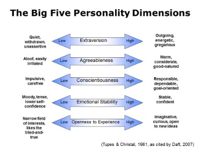
As part of this exploratory study, I intend to examine the potential role that Big 5 personality variables (i.e., openness to new experience, neuroticism, extraversion, conscientiousness, agreeableness) play in people's propensity to believe in or accept generic conspiracist beliefs, (as well as to the five factors produced by the GCBS (i.e., government malfeasance, extraterrestrial cover-up, malevolent global, personal well-being, control of information). Generally, which personality trait is most likely to be related to generic conspiracist beliefs, and how might that related to other variables such as age, gender, and religious orientation.
As I claimed in the introduction, conspiracy beliefs—with which Big 5 personality traits is likely to be associated—have led to differences in how people and states have reacted—not only to the COVID-19 pandemic—but also to other conspiracy theory-laden events, such as the 2020 presidential elections.
However, my previously mentioned individual-level dataset is limited in that it does not collect data on regioinal location of its participants. As I will describe for you soon, in order to answer my research questions related to state-level personality and conspiracist beliefs, I collected state-level data from three different data sources providing state-level Big-5 personality trait averages, along with other state-level variables including beliefs in specific conspiracy theory narratives and states' level of restrictedness in dealing with the pandemic.
To summarize, by the end of this tutorial, I hope to answer my research questions:
I.) Individual-level Dataset: As mentioned previously, these data come from an open-source dataset on kaggle.com that collects measures of generic conspiracist beliefs, Big 5 traits, and other demographic measures.
Click here to go to section on ETL processing for this particular dataset.
This dataset is intended to be used to answer the research questions: "How do Big-5 personality traits relate to people's general inclinations toward conspiracist beliefs?", & "If there is an assocation, what type of unique effect does Openness have on those beliefs?".
II.) State-level Big-5 Averages: I initially procured these data off of a Wikipedia page that provided information from the following paper by Renfrow, Gosling, and Potter published in 2008 in Psychological Science. The first author, Dr. Peter J. Rentfrow, is well-known for his research in regionally-clustered psychological traits.
The Wikipedia page, as well as the published paper only provided standardized state means, state ranking, and sample sizes for each of the 50 US states and Washington D.C across all five personality traits.. I followed up with Dr. Rentfrow via e-mail who provided me with a .csv file of the raw means and standard deviations of their data (see State Means and SDs.csv in my GitHub website).
Click here to go to section on ETL processing for this particular dataset.
III.) State-level Beliefs in Conspiracy Theories: Given the novelty of the Generic Conspiracist Beliefs Scale, there were no state-level dataset (or individual-level dataset that could be aggregated by state) in order to mirror the Individual-level Dataset.
So, I searched through data collected in 2020 by the American National Election Studies (ANES). The ANES collects indiviudal-level data in the United States annually. Their survey data provide information on perceptions of different political candidates, social issues, and—as part of their 2020 wave—beliefs about various specific false narratives, which serve as a proxy to conspiracist beliefs for the purposes of my research questions. Examples of these narratives ask participants the extent to which they believe that vaccines cause autism or that COVID-19 was intentionally developed in a laboratory.
I computed mean state-level variables by first grouping by state and then computing the mean composite. In addition to beliefs in false narratives, I retained state-level demographic variabels to control for like state-level political conservatism and highest level of education.
Click here to go to section on ETL processing for this particular dataset.
IV.) State-Level Non-Restrictive Responses to COVID-19 Indices: These data were collected on Wallethub.com from a table that scored all 50 US states and Washington D.C. on how least restrictive they were in response to the COVID-19 pandemic. In order to calculate state scores, 13 metrics were used using a scale from 1 to 100, with 100 indicating states that had the least restrictions. Metrics included states that did not require mask-wearing to states that prohibited large gatherings. Please read more about how these scores were calculated here.
Click here to go to section on ETL processing for this particular dataset.
II.) State-level Big-5 Averages,III.) State-level Beliefs in Conspiracy Theories, andIV.) State-Level Non-Restrictive Responses to COVID-19 Indiceswere merged to create my state-level dataset. Click here to go to the section on ETL processing for this particular dataset.This dataset was used explore the last two research questions: At the state-level, how does personality—data from
II.) State-level Big-5 Averages)—relate to attitudes toward specific conspiracy beliefs—(data fromIII.) State-level Beliefs in Conspiracy Theories)? & How does this relationship impact states' varied responses to the COVID-19 pandemic—(data fromIV.) State-Level Non-Restrictive Responses to COVID-19 Indices)?
As might be evident in my second research question, I am actually predicting that Openness to New Experiences might be the one Big Five trait that significantly related to generic conspiracist beliefs. Why? I imagine people who are high in Openness are more open to considering alternative narratives relative to people low in Openness. This might also translate at the state level and impact how different states responded to the COVID-19 pandemic.
The other Big Five traits may be related to generic conspiracist beliefs but in a less significant way. However, these secondary analyses are exploratory in nature, so all traits will be investigated.
Here are all the packages and libraries that I used for this tutorial.
#Load dataset and parse into shape using principles of tidy data.
%matplotlib inline
!pip3 install lxml
!pip3 install pingouin
!pip3 install scikit-posthocs
!pip install chart_studio
import chart_studio.plotly as py
import plotly.graph_objects as go
import plotly.express as px
import pingouin as pg
import matplotlib.pyplot as plt
import matplotlib.ticker as ticker
import scipy
import scipy.stats as sp
from scipy.stats import mstats
from scipy.stats import ttest_ind
import scikit_posthocs as scikit
from sklearn.neighbors import KNeighborsRegressor
from sklearn.preprocessing import StandardScaler
import seaborn as sns
import statsmodels.api as sm
import statsmodels.formula.api as sfa
from statsmodels.formula.api import ols
import scikit_posthocs as scikit
from bs4 import BeautifulSoup as bs
import lxml
import pandas as pd
import numpy as np
import requests as requests
# Widens the notebook and lets us display data easily.
from IPython.core.display import display, HTML
display(HTML("<style>.container { width:95% !important; }</style>"))
# Show a very large number of rows and columns
pd.set_option('display.max_rows', 500)
pd.set_option('display.max_columns', 500)
pd.set_option('display.width', 1000)
Collecting lxml
Downloading lxml-4.7.1-cp39-cp39-manylinux_2_17_x86_64.manylinux2014_x86_64.manylinux_2_24_x86_64.whl (6.9 MB)
|████████████████████████████████| 6.9 MB 2.2 MB/s eta 0:00:01
Installing collected packages: lxml
Successfully installed lxml-4.7.1
Collecting pingouin
Downloading pingouin-0.5.0.tar.gz (182 kB)
|████████████████████████████████| 182 kB 2.3 MB/s eta 0:00:01
Requirement already satisfied: numpy>=1.19 in /opt/conda/lib/python3.9/site-packages (from pingouin) (1.20.3)
Requirement already satisfied: scipy>=1.7 in /opt/conda/lib/python3.9/site-packages (from pingouin) (1.7.1)
Requirement already satisfied: pandas>=1.0 in /opt/conda/lib/python3.9/site-packages (from pingouin) (1.3.3)
Requirement already satisfied: matplotlib>=3.0.2 in /opt/conda/lib/python3.9/site-packages (from pingouin) (3.4.3)
Requirement already satisfied: seaborn>=0.9.0 in /opt/conda/lib/python3.9/site-packages (from pingouin) (0.11.2)
Requirement already satisfied: statsmodels>=0.12.0 in /opt/conda/lib/python3.9/site-packages (from pingouin) (0.12.2)
Requirement already satisfied: scikit-learn in /opt/conda/lib/python3.9/site-packages (from pingouin) (0.24.2)
Collecting pandas_flavor>=0.2.0
Downloading pandas_flavor-0.2.0-py2.py3-none-any.whl (6.6 kB)
Collecting outdated
Downloading outdated-0.2.1-py3-none-any.whl (7.5 kB)
Collecting tabulate
Downloading tabulate-0.8.9-py3-none-any.whl (25 kB)
Requirement already satisfied: pyparsing>=2.2.1 in /opt/conda/lib/python3.9/site-packages (from matplotlib>=3.0.2->pingouin) (2.4.7)
Requirement already satisfied: kiwisolver>=1.0.1 in /opt/conda/lib/python3.9/site-packages (from matplotlib>=3.0.2->pingouin) (1.3.2)
Requirement already satisfied: pillow>=6.2.0 in /opt/conda/lib/python3.9/site-packages (from matplotlib>=3.0.2->pingouin) (8.3.2)
Requirement already satisfied: cycler>=0.10 in /opt/conda/lib/python3.9/site-packages (from matplotlib>=3.0.2->pingouin) (0.10.0)
Requirement already satisfied: python-dateutil>=2.7 in /opt/conda/lib/python3.9/site-packages (from matplotlib>=3.0.2->pingouin) (2.8.2)
Requirement already satisfied: six in /opt/conda/lib/python3.9/site-packages (from cycler>=0.10->matplotlib>=3.0.2->pingouin) (1.16.0)
Requirement already satisfied: pytz>=2017.3 in /opt/conda/lib/python3.9/site-packages (from pandas>=1.0->pingouin) (2021.1)
Collecting xarray
Downloading xarray-0.20.2-py3-none-any.whl (845 kB)
|████████████████████████████████| 845 kB 13.8 MB/s eta 0:00:01
Requirement already satisfied: patsy>=0.5 in /opt/conda/lib/python3.9/site-packages (from statsmodels>=0.12.0->pingouin) (0.5.1)
Collecting littleutils
Downloading littleutils-0.2.2.tar.gz (6.6 kB)
Requirement already satisfied: requests in /opt/conda/lib/python3.9/site-packages (from outdated->pingouin) (2.26.0)
Requirement already satisfied: charset-normalizer~=2.0.0 in /opt/conda/lib/python3.9/site-packages (from requests->outdated->pingouin) (2.0.0)
Requirement already satisfied: idna<4,>=2.5 in /opt/conda/lib/python3.9/site-packages (from requests->outdated->pingouin) (3.1)
Requirement already satisfied: urllib3<1.27,>=1.21.1 in /opt/conda/lib/python3.9/site-packages (from requests->outdated->pingouin) (1.26.6)
Requirement already satisfied: certifi>=2017.4.17 in /opt/conda/lib/python3.9/site-packages (from requests->outdated->pingouin) (2021.5.30)
Requirement already satisfied: threadpoolctl>=2.0.0 in /opt/conda/lib/python3.9/site-packages (from scikit-learn->pingouin) (2.2.0)
Requirement already satisfied: joblib>=0.11 in /opt/conda/lib/python3.9/site-packages (from scikit-learn->pingouin) (1.0.1)
Building wheels for collected packages: pingouin, littleutils
Building wheel for pingouin (setup.py) ... done
Created wheel for pingouin: filename=pingouin-0.5.0-py3-none-any.whl size=193661 sha256=c4afb344049347f197d4b068b2109498ffb7795d64e994974c061d92bdbab6b7
Stored in directory: /home/jovyan/.cache/pip/wheels/ac/42/e9/bd0edc18701d9b7ab4b09be127909823f131054f35373abc0c
Building wheel for littleutils (setup.py) ... done
Created wheel for littleutils: filename=littleutils-0.2.2-py3-none-any.whl size=7048 sha256=a6c639d3f2cd543d69f745c8736d05060adaf9fe65f8658ad88230be6590e4ec
Stored in directory: /home/jovyan/.cache/pip/wheels/04/bb/0d/2d02ec45f29c48d6192476bfb59c5a0e64b605e7212374dd15
Successfully built pingouin littleutils
Installing collected packages: xarray, littleutils, tabulate, pandas-flavor, outdated, pingouin
Successfully installed littleutils-0.2.2 outdated-0.2.1 pandas-flavor-0.2.0 pingouin-0.5.0 tabulate-0.8.9 xarray-0.20.2
Collecting scikit-posthocs
Downloading scikit-posthocs-0.6.7.tar.gz (43 kB)
|████████████████████████████████| 43 kB 696 kB/s eta 0:00:01
Installing build dependencies ... done
Getting requirements to build wheel ... done
Preparing wheel metadata ... done
Requirement already satisfied: numpy in /opt/conda/lib/python3.9/site-packages (from scikit-posthocs) (1.20.3)
Requirement already satisfied: pandas>=0.20.0 in /opt/conda/lib/python3.9/site-packages (from scikit-posthocs) (1.3.3)
Requirement already satisfied: statsmodels in /opt/conda/lib/python3.9/site-packages (from scikit-posthocs) (0.12.2)
Requirement already satisfied: matplotlib in /opt/conda/lib/python3.9/site-packages (from scikit-posthocs) (3.4.3)
Requirement already satisfied: scipy in /opt/conda/lib/python3.9/site-packages (from scikit-posthocs) (1.7.1)
Requirement already satisfied: seaborn in /opt/conda/lib/python3.9/site-packages (from scikit-posthocs) (0.11.2)
Requirement already satisfied: python-dateutil>=2.7.3 in /opt/conda/lib/python3.9/site-packages (from pandas>=0.20.0->scikit-posthocs) (2.8.2)
Requirement already satisfied: pytz>=2017.3 in /opt/conda/lib/python3.9/site-packages (from pandas>=0.20.0->scikit-posthocs) (2021.1)
Requirement already satisfied: six>=1.5 in /opt/conda/lib/python3.9/site-packages (from python-dateutil>=2.7.3->pandas>=0.20.0->scikit-posthocs) (1.16.0)
Requirement already satisfied: kiwisolver>=1.0.1 in /opt/conda/lib/python3.9/site-packages (from matplotlib->scikit-posthocs) (1.3.2)
Requirement already satisfied: cycler>=0.10 in /opt/conda/lib/python3.9/site-packages (from matplotlib->scikit-posthocs) (0.10.0)
Requirement already satisfied: pillow>=6.2.0 in /opt/conda/lib/python3.9/site-packages (from matplotlib->scikit-posthocs) (8.3.2)
Requirement already satisfied: pyparsing>=2.2.1 in /opt/conda/lib/python3.9/site-packages (from matplotlib->scikit-posthocs) (2.4.7)
Requirement already satisfied: patsy>=0.5 in /opt/conda/lib/python3.9/site-packages (from statsmodels->scikit-posthocs) (0.5.1)
Building wheels for collected packages: scikit-posthocs
Building wheel for scikit-posthocs (PEP 517) ... done
Created wheel for scikit-posthocs: filename=scikit_posthocs-0.6.7-py3-none-any.whl size=37902 sha256=d2f5f304995b074129b5d39460637b5405d50e906fe3ca880aab6ecff71f87ae
Stored in directory: /home/jovyan/.cache/pip/wheels/9d/b3/0e/48fc4edf03f0cace0bb10215f6103591b62f143ace946c193c
Successfully built scikit-posthocs
Installing collected packages: scikit-posthocs
Successfully installed scikit-posthocs-0.6.7
Collecting chart_studio
Downloading chart_studio-1.1.0-py3-none-any.whl (64 kB)
|████████████████████████████████| 64 kB 1.5 MB/s eta 0:00:01
Collecting plotly
Downloading plotly-5.4.0-py2.py3-none-any.whl (25.3 MB)
|████████████████████████████████| 25.3 MB 16.9 MB/s eta 0:00:01 |███████████ | 8.7 MB 4.2 MB/s eta 0:00:04
Requirement already satisfied: six in /opt/conda/lib/python3.9/site-packages (from chart_studio) (1.16.0)
Requirement already satisfied: requests in /opt/conda/lib/python3.9/site-packages (from chart_studio) (2.26.0)
Collecting retrying>=1.3.3
Downloading retrying-1.3.3.tar.gz (10 kB)
Collecting tenacity>=6.2.0
Downloading tenacity-8.0.1-py3-none-any.whl (24 kB)
Requirement already satisfied: idna<4,>=2.5 in /opt/conda/lib/python3.9/site-packages (from requests->chart_studio) (3.1)
Requirement already satisfied: charset-normalizer~=2.0.0 in /opt/conda/lib/python3.9/site-packages (from requests->chart_studio) (2.0.0)
Requirement already satisfied: certifi>=2017.4.17 in /opt/conda/lib/python3.9/site-packages (from requests->chart_studio) (2021.5.30)
Requirement already satisfied: urllib3<1.27,>=1.21.1 in /opt/conda/lib/python3.9/site-packages (from requests->chart_studio) (1.26.6)
Building wheels for collected packages: retrying
Building wheel for retrying (setup.py) ... done
Created wheel for retrying: filename=retrying-1.3.3-py3-none-any.whl size=11448 sha256=e1b343f35eb296b72b197ff514ecbec56f33233647d4cba4a84c8f1352626e0a
Stored in directory: /home/jovyan/.cache/pip/wheels/ce/18/7f/e9527e3e66db1456194ac7f61eb3211068c409edceecff2d31
Successfully built retrying
Installing collected packages: tenacity, retrying, plotly, chart-studio
Successfully installed chart-studio-1.1.0 plotly-5.4.0 retrying-1.3.3 tenacity-8.0.1
$\color{blue}{\text{In the following section, I will take you through how I extracted and preprocessed the various datasets, as well as calculated composite scores where appropropriate.}}$
Click here to go to top of page.
The first goal was to create a new DataFrame with the individual-level variables of relevance from this open dataset. On the following website, I accessed the data my clicking on a link and downloading a .csv file of the raw data. Dataset saved in my GitHub website under "conspiracy_data.csv". I also dropped several columns representing variables that were not relevant to my research questions, nor were variables I thought would be important to control for.
# Get kaggle webpage that contains csv file with data
url = "https://www.kaggle.com/yamqwe/measuring-belief-in-conspiracy-theories"
r = requests.get(url)
r.status_code
200
# Manually downloaded csv data onto Docker as dataset can only be downloaded once link on website is clicked.
# Dataset is saved in my GitHub.
conspiracy_df = pd.read_csv("conspiracy_data.csv")
conspiracy_df.head()
conspiracy_df.shape # There are 2495 rows (participants) and 72 columns (variables).
# Drop column/variable as it is not relevant to research questions.
conspiracy_df = conspiracy_df.drop(["major"], axis=1)
conspiracy_df = conspiracy_df.drop(["E1","E2","E3","E4","E5","E6","E7","E8","E9","E10","E11","E12","E13","E14","E15",
"introelapse", "testelapse", "surveyelapse",
"VCL1", "VCL2", "VCL3", "VCL4", "VCL5", "VCL7", "VCL8", "VCL10", "VCL11", "VCL13", "VCL14", "VCL15", "VCL16",
"introelapse", "testelapse", "surveyelapse",
"urban", "hand", "orientation", "race", "married", "familysize"], axis=1)
conspiracy_df # There are 2495 rows (participants) and 72 columns (variables).
conspiracy_df.engnat.value_counts() # There are 1875 participants who identified as native English speakers, 612, non-native, and 8 no responses.
pd.set_option('display.max_rows', 10)
conspiracy_df.head()
| Q1 | Q2 | Q3 | Q4 | Q5 | Q6 | Q7 | Q8 | Q9 | Q10 | Q11 | Q12 | Q13 | Q14 | Q15 | TIPI1 | TIPI2 | TIPI3 | TIPI4 | TIPI5 | TIPI6 | TIPI7 | TIPI8 | TIPI9 | TIPI10 | VCL6 | VCL9 | VCL12 | education | gender | engnat | age | religion | voted | |
|---|---|---|---|---|---|---|---|---|---|---|---|---|---|---|---|---|---|---|---|---|---|---|---|---|---|---|---|---|---|---|---|---|---|---|
| 0 | 5 | 5 | 3 | 5 | 5 | 5 | 5 | 3 | 4 | 5 | 5 | 5 | 3 | 5 | 5 | 5 | 3 | 6 | 2 | 6 | 6 | 7 | 2 | 7 | 1 | 0 | 0 | 0 | 3 | 1 | 2 | 28 | 2 | 2 |
| 1 | 5 | 5 | 5 | 5 | 5 | 3 | 5 | 5 | 1 | 4 | 4 | 5 | 4 | 4 | 5 | 6 | 7 | 6 | 7 | 6 | 3 | 7 | 5 | 1 | 1 | 0 | 0 | 0 | 1 | 2 | 1 | 14 | 1 | 2 |
| 2 | 2 | 4 | 1 | 2 | 2 | 2 | 4 | 2 | 2 | 4 | 2 | 4 | 0 | 2 | 4 | 6 | 6 | 6 | 1 | 7 | 5 | 6 | 5 | 7 | 7 | 1 | 0 | 0 | 4 | 2 | 2 | 26 | 1 | 1 |
| 3 | 5 | 4 | 1 | 2 | 4 | 5 | 4 | 1 | 4 | 5 | 5 | 5 | 1 | 4 | 5 | 6 | 7 | 7 | 5 | 7 | 6 | 5 | 1 | 5 | 1 | 0 | 0 | 0 | 3 | 1 | 1 | 25 | 12 | 1 |
| 4 | 5 | 4 | 1 | 4 | 4 | 5 | 4 | 3 | 1 | 5 | 5 | 5 | 3 | 5 | 5 | 1 | 3 | 7 | 2 | 6 | 4 | 5 | 5 | 5 | 3 | 0 | 0 | 0 | 2 | 1 | 1 | 37 | 2 | 2 |
The following code checked each column to determine if there were any NaN values, the dtypes for each column, and if any columns had a value of zero, which would have indicated that participants did not respond to that item.
# Output number of columns with 'NaN' values to determine if participants should be eliminated from analyses due to substantial incomplete responses.
conspiracy_df.info() # All columns are integers and do not contain 'NaN' values.
# Check to ensure there are no 0 values for scale items whose choice options are greater than 0.
# This means participant did not respond to item.
conspiracy_df.min()
<class 'pandas.core.frame.DataFrame'> RangeIndex: 2495 entries, 0 to 2494 Data columns (total 34 columns): # Column Non-Null Count Dtype --- ------ -------------- ----- 0 Q1 2495 non-null int64 1 Q2 2495 non-null int64 2 Q3 2495 non-null int64 3 Q4 2495 non-null int64 4 Q5 2495 non-null int64 5 Q6 2495 non-null int64 6 Q7 2495 non-null int64 7 Q8 2495 non-null int64 8 Q9 2495 non-null int64 9 Q10 2495 non-null int64 10 Q11 2495 non-null int64 11 Q12 2495 non-null int64 12 Q13 2495 non-null int64 13 Q14 2495 non-null int64 14 Q15 2495 non-null int64 15 TIPI1 2495 non-null int64 16 TIPI2 2495 non-null int64 17 TIPI3 2495 non-null int64 18 TIPI4 2495 non-null int64 19 TIPI5 2495 non-null int64 20 TIPI6 2495 non-null int64 21 TIPI7 2495 non-null int64 22 TIPI8 2495 non-null int64 23 TIPI9 2495 non-null int64 24 TIPI10 2495 non-null int64 25 VCL6 2495 non-null int64 26 VCL9 2495 non-null int64 27 VCL12 2495 non-null int64 28 education 2495 non-null int64 29 gender 2495 non-null int64 30 engnat 2495 non-null int64 31 age 2495 non-null int64 32 religion 2495 non-null int64 33 voted 2495 non-null int64 dtypes: int64(34) memory usage: 662.9 KB
Q1 0
Q2 0
Q3 0
Q4 0
Q5 0
..
gender 0
engnat 0
age 13
religion 0
voted 0
Length: 34, dtype: int64
The next cells contain code that created a DataFrame of the columns or items that would eventually be used to compute mean composite scores for the Generic Conspiracist Beliefs Scale (GCBS) and the Big 5 traits in order to mean impute values of '0'. Next, the non-scale items were merged into the new DataFrame.
# Create new DataFrame with only scale items in order to mean impute zero values, which were blank responses from participants.
# 2495 rows and 34 columns.
conspiracy_scale_items_df = conspiracy_df[["Q1","Q2","Q3","Q4","Q5","Q6","Q7","Q8","Q9","Q10","Q11","Q12","Q13","Q14","Q15",
"TIPI1","TIPI2","TIPI3","TIPI4","TIPI5","TIPI6","TIPI7","TIPI8","TIPI9","TIPI10"]].copy()
conspiracy_scale_items_df.replace(0,conspiracy_scale_items_df.mean(axis=0),inplace=True)
# Drop old columns from original DataFrame and renamed as new DataFrame
conspiracy_df_1 = conspiracy_df.drop(columns=["Q1","Q2","Q3","Q4","Q5","Q6","Q7","Q8","Q9","Q10","Q11","Q12","Q13","Q14","Q15",
"TIPI1","TIPI2","TIPI3","TIPI4","TIPI5","TIPI6","TIPI7","TIPI8","TIPI9","TIPI10"])
(conspiracy_df_1)
# Merge both DataFrames.
conspiracy_scale_items_df["VCL6"] = conspiracy_df_1["VCL6"]
conspiracy_scale_items_df["VCL9"] = conspiracy_df_1["VCL9"]
conspiracy_scale_items_df["VCL12"] = conspiracy_df_1["VCL12"]
conspiracy_scale_items_df["education"] = conspiracy_df_1["education"]
conspiracy_scale_items_df["gender"] = conspiracy_df_1["gender"]
conspiracy_scale_items_df["engnat"] = conspiracy_df_1["engnat"]
conspiracy_scale_items_df["age"] = conspiracy_df_1["age"]
conspiracy_scale_items_df["religion"] = conspiracy_df_1["religion"]
conspiracy_scale_items_df["voted"] = conspiracy_df_1["voted"]
conspiracy_scale_items_df['Q10'] = conspiracy_scale_items_df['Q10'].astype(float)
conspiracy_scale_items_df.head()
| Q1 | Q2 | Q3 | Q4 | Q5 | Q6 | Q7 | Q8 | Q9 | Q10 | Q11 | Q12 | Q13 | Q14 | Q15 | TIPI1 | TIPI2 | TIPI3 | TIPI4 | TIPI5 | TIPI6 | TIPI7 | TIPI8 | TIPI9 | TIPI10 | VCL6 | VCL9 | VCL12 | education | gender | engnat | age | religion | voted | |
|---|---|---|---|---|---|---|---|---|---|---|---|---|---|---|---|---|---|---|---|---|---|---|---|---|---|---|---|---|---|---|---|---|---|---|
| 0 | 5.0 | 5.0 | 3.0 | 5.0 | 5.0 | 5.0 | 5.0 | 3.0 | 4.0 | 5.0 | 5.0 | 5.0 | 3.000000 | 5.0 | 5.0 | 5.0 | 3.0 | 6.0 | 2.0 | 6.0 | 6.0 | 7.0 | 2.0 | 7.0 | 1.0 | 0 | 0 | 0 | 3 | 1 | 2 | 28 | 2 | 2 |
| 1 | 5.0 | 5.0 | 5.0 | 5.0 | 5.0 | 3.0 | 5.0 | 5.0 | 1.0 | 4.0 | 4.0 | 5.0 | 4.000000 | 4.0 | 5.0 | 6.0 | 7.0 | 6.0 | 7.0 | 6.0 | 3.0 | 7.0 | 5.0 | 1.0 | 1.0 | 0 | 0 | 0 | 1 | 2 | 1 | 14 | 1 | 2 |
| 2 | 2.0 | 4.0 | 1.0 | 2.0 | 2.0 | 2.0 | 4.0 | 2.0 | 2.0 | 4.0 | 2.0 | 4.0 | 2.103006 | 2.0 | 4.0 | 6.0 | 6.0 | 6.0 | 1.0 | 7.0 | 5.0 | 6.0 | 5.0 | 7.0 | 7.0 | 1 | 0 | 0 | 4 | 2 | 2 | 26 | 1 | 1 |
| 3 | 5.0 | 4.0 | 1.0 | 2.0 | 4.0 | 5.0 | 4.0 | 1.0 | 4.0 | 5.0 | 5.0 | 5.0 | 1.000000 | 4.0 | 5.0 | 6.0 | 7.0 | 7.0 | 5.0 | 7.0 | 6.0 | 5.0 | 1.0 | 5.0 | 1.0 | 0 | 0 | 0 | 3 | 1 | 1 | 25 | 12 | 1 |
| 4 | 5.0 | 4.0 | 1.0 | 4.0 | 4.0 | 5.0 | 4.0 | 3.0 | 1.0 | 5.0 | 5.0 | 5.0 | 3.000000 | 5.0 | 5.0 | 1.0 | 3.0 | 7.0 | 2.0 | 6.0 | 4.0 | 5.0 | 5.0 | 5.0 | 3.0 | 0 | 0 | 0 | 2 | 1 | 1 | 37 | 2 | 2 |
The following cells contain code that renames columns so that their variable name relates to the factor found in the scale items. For example, I renamed items Q1 to Q15, which were the Generic Conspiracist belief items, to "GCBS_gm_1 to GCBS_ci_15. Note that the GCBS scale has five factors along with the global composite, i.e., all items in the scale, that can be calculated as composite means. The focus of this tutorial is to look at the global score, however the renamed items reflect the GCBS factors as well for future exploratory research.
The Big Five traits were calculated using the Ten Item Personality Inventory or TIPI. Each Big Five factor is made up of two items, however items 2, 6, 8, 9, 10 required reverse coding, which I conducted using the .map() function. The original items are preserved, and new variables are created with the reverse coding enacted.
Lastly, participants were dropped from this dataset who failed the validity checks in the survey. Final sample size is 2234 participants.
# Change column/variable names
# Q1 - Q15 consist of the GCBS.
conspiracy_scale_items_df = conspiracy_scale_items_df.rename(columns={"Q1":"GCBS_gm_1","Q2":"GCBS_mgc_2", "Q3":"GCBS_ec_3","Q4":"GCBS_pw_4", "Q5":"GCBS_ci_5",
"Q6":"GCBS_gm_6", "Q7":"GCBS_mgc_7", "Q8":"GCBS_ec_8", "Q9":"GCBS_pw_9","Q10":"GCBS_ci_10",
"Q11":"GCBS_gm_11", "Q12":"GCBS_mgc_12", "Q13":"GCBS_ec_13", "Q14":"GCBS_pw_14", "Q15":"GCBS_ci_15"})
# Rename TIPI1 to TIPI15 to determine which items belong to which factors.
conspiracy_scale_items_df = conspiracy_scale_items_df.rename(columns={"TIPI1":"TIPI1_e", "TIPI2":"TIPI2_a", "TIPI3":"TIPI3_c", "TIPI4":"TIPI4_n", "TIPI5":"TIPI5_o",
"TIPI6":"TIPI6_e" , "TIPI7":"TIPI7_a", "TIPI8":"TIPI8_c" , "TIPI9":"TIPI9_n" , "TIPI10":"TIPI10_o"})
# Create new columns/variables with items 6, 2, 8, 9, 10 recoded.
conspiracy_scale_items_df["TIPI6_e_r"] = conspiracy_scale_items_df["TIPI6_e"].map({1:7, 2:6, 3:5, 4:4, 5:3, 6:2, 7:1})
conspiracy_scale_items_df["TIPI2_a_r"] = conspiracy_scale_items_df["TIPI2_a"].map({1:7, 2:6, 3:5, 4:4, 5:3, 6:2, 7:1})
conspiracy_scale_items_df["TIPI8_c_r"] = conspiracy_scale_items_df["TIPI8_c"].map({1:7, 2:6, 3:5, 4:4, 5:3, 6:2, 7:1})
conspiracy_scale_items_df["TIPI9_n_r"] = conspiracy_scale_items_df["TIPI9_n"].map({1:7, 2:6, 3:5, 4:4, 5:3, 6:2, 7:1})
conspiracy_scale_items_df["TIPI10_o_r"] = conspiracy_scale_items_df["TIPI10_o"].map({1:7, 2:6, 3:5, 4:4, 5:3, 6:2, 7:1})
# Drop the following rows/participants from analyses (Total N = 2495).
# Participants who failed validity checks.
conspiracy_scale_items_df["VCL6"].value_counts() # Passed = 2234, Failed = 261
conspiracy_scale_items_df["VCL9"].value_counts() # Passed = 2347, Failed = 148
conspiracy_scale_items_df["VCL12"].value_counts() # Passed = 2078, Failed = 417
conspiracy_scale_items_df = conspiracy_scale_items_df[(conspiracy_scale_items_df.VCL6 != 1) | (conspiracy_scale_items_df.VCL6 != 1) | (conspiracy_scale_items_df.VCL6 != 1)]
conspiracy_scale_items_df.head() #Total N = 2234
| GCBS_gm_1 | GCBS_mgc_2 | GCBS_ec_3 | GCBS_pw_4 | GCBS_ci_5 | GCBS_gm_6 | GCBS_mgc_7 | GCBS_ec_8 | GCBS_pw_9 | GCBS_ci_10 | GCBS_gm_11 | GCBS_mgc_12 | GCBS_ec_13 | GCBS_pw_14 | GCBS_ci_15 | TIPI1_e | TIPI2_a | TIPI3_c | TIPI4_n | TIPI5_o | TIPI6_e | TIPI7_a | TIPI8_c | TIPI9_n | TIPI10_o | VCL6 | VCL9 | VCL12 | education | gender | engnat | age | religion | voted | TIPI6_e_r | TIPI2_a_r | TIPI8_c_r | TIPI9_n_r | TIPI10_o_r | |
|---|---|---|---|---|---|---|---|---|---|---|---|---|---|---|---|---|---|---|---|---|---|---|---|---|---|---|---|---|---|---|---|---|---|---|---|---|---|---|---|
| 0 | 5.0 | 5.0 | 3.0 | 5.0 | 5.0 | 5.0 | 5.0 | 3.0 | 4.0 | 5.0 | 5.0 | 5.0 | 3.0 | 5.0 | 5.0 | 5.0 | 3.0 | 6.0 | 2.0 | 6.0 | 6.0 | 7.0 | 2.0 | 7.0 | 1.0 | 0 | 0 | 0 | 3 | 1 | 2 | 28 | 2 | 2 | 2.0 | 5.0 | 6.0 | 1.0 | 7.0 |
| 1 | 5.0 | 5.0 | 5.0 | 5.0 | 5.0 | 3.0 | 5.0 | 5.0 | 1.0 | 4.0 | 4.0 | 5.0 | 4.0 | 4.0 | 5.0 | 6.0 | 7.0 | 6.0 | 7.0 | 6.0 | 3.0 | 7.0 | 5.0 | 1.0 | 1.0 | 0 | 0 | 0 | 1 | 2 | 1 | 14 | 1 | 2 | 5.0 | 1.0 | 3.0 | 7.0 | 7.0 |
| 3 | 5.0 | 4.0 | 1.0 | 2.0 | 4.0 | 5.0 | 4.0 | 1.0 | 4.0 | 5.0 | 5.0 | 5.0 | 1.0 | 4.0 | 5.0 | 6.0 | 7.0 | 7.0 | 5.0 | 7.0 | 6.0 | 5.0 | 1.0 | 5.0 | 1.0 | 0 | 0 | 0 | 3 | 1 | 1 | 25 | 12 | 1 | 2.0 | 1.0 | 7.0 | 3.0 | 7.0 |
| 4 | 5.0 | 4.0 | 1.0 | 4.0 | 4.0 | 5.0 | 4.0 | 3.0 | 1.0 | 5.0 | 5.0 | 5.0 | 3.0 | 5.0 | 5.0 | 1.0 | 3.0 | 7.0 | 2.0 | 6.0 | 4.0 | 5.0 | 5.0 | 5.0 | 3.0 | 0 | 0 | 0 | 2 | 1 | 1 | 37 | 2 | 2 | 4.0 | 5.0 | 3.0 | 3.0 | 5.0 |
| 5 | 1.0 | 1.0 | 1.0 | 1.0 | 1.0 | 1.0 | 1.0 | 1.0 | 1.0 | 1.0 | 1.0 | 1.0 | 1.0 | 1.0 | 1.0 | 4.0 | 2.0 | 6.0 | 2.0 | 6.0 | 5.0 | 6.0 | 3.0 | 6.0 | 2.0 | 0 | 1 | 1 | 3 | 1 | 1 | 34 | 7 | 1 | 3.0 | 6.0 | 5.0 | 2.0 | 6.0 |
The following code contains code that computes mean composite scores for the Global GCBS and each factor of the Big Five Inventory. Note that the following code also computes mean composites for the five factors of GCBS, but that is meant for future exploratory research as is not pertinent to the current research questions.
Before computing composite scores, I conducted reliablity checks of the scale items by calculating Cronbach's alpha using the pingouin package and .cronbach_alpha() function. Note that conventional cutoffs for Cronbach's alpha typically fall at .70, however the much lower alpha's for Agreeableness and Openness may be expected due to the fact that each factor is composed of only two items, and number of items can impact Cronbach's alpha.
## GENERIC CONSPIRACIST BELIEFS SCALE ##
# GLOBAL GCBS #
# Reliablity check for Global GCBS measure, a = 0.93
Global_GCBS_alpha = pg.cronbach_alpha(data=conspiracy_scale_items_df[["GCBS_gm_1","GCBS_mgc_2","GCBS_ec_3","GCBS_pw_4","GCBS_ci_5",
"GCBS_gm_6","GCBS_mgc_7","GCBS_ec_8","GCBS_pw_9","GCBS_ci_10",
"GCBS_gm_11","GCBS_mgc_12","GCBS_ec_13","GCBS_pw_14","GCBS_ci_15"]])
# Compute Global GCBS composite.
conspiracy_scale_items_df['Global_GCBS'] = conspiracy_scale_items_df[["GCBS_gm_1","GCBS_mgc_2","GCBS_ec_3","GCBS_pw_4","GCBS_ci_5",
"GCBS_gm_6","GCBS_mgc_7","GCBS_ec_8","GCBS_pw_9","GCBS_ci_10",
"GCBS_gm_11","GCBS_mgc_12","GCBS_ec_13","GCBS_pw_14","GCBS_ci_15"]].mean(axis=1)
# Reliability check for GCBS Factor 1, Government Malfeasance, a = .84
GCBS_Gov_Mal_alpha = pg.cronbach_alpha(data=conspiracy_scale_items_df[["GCBS_gm_1","GCBS_gm_6","GCBS_gm_11"]])
# Compute GCBS Government Malfeasance composite.
conspiracy_scale_items_df["GCBS_Gov_Mal"] = conspiracy_scale_items_df[["GCBS_gm_1","GCBS_gm_6","GCBS_gm_11"]].mean(axis=1)
# Reliability check for GCBS Factor 2, Malevolent Global Conspiracies, a = .89
GCBS_Mal_Global_alpha = pg.cronbach_alpha(data=conspiracy_scale_items_df[["GCBS_mgc_2","GCBS_mgc_7","GCBS_mgc_12"]])
# Compute GCBS Malevolent Global Conspiracies composite.
conspiracy_scale_items_df["GCBS_Mal_Global"] = conspiracy_scale_items_df[["GCBS_mgc_2","GCBS_mgc_7","GCBS_mgc_12"]].mean(axis=1)
# Reliability check for GCBS Factor 3, Extraterrestrial Cover-Up, a = .90
GCBS_Extra_Cover_alpha = pg.cronbach_alpha(data=conspiracy_scale_items_df[["GCBS_ec_3","GCBS_ec_8","GCBS_ec_13"]])
# Compute GCBS Extraterrestrial Cover-Up composite.
conspiracy_scale_items_df["GCBS_Extra_Cover"] = conspiracy_scale_items_df[["GCBS_ec_3","GCBS_ec_8","GCBS_ec_13"]].mean(axis=1)
# Reliability check for GCBS Factor 4, Personal Well-Being, a = .81
GCBS_Person_Well_alpha = pg.cronbach_alpha(data=conspiracy_scale_items_df[["GCBS_pw_4","GCBS_pw_9","GCBS_pw_14"]])
# Compute GCBS Personal Well-Being composite.
conspiracy_scale_items_df["GCBS_Person_Well"] = conspiracy_scale_items_df[["GCBS_pw_4","GCBS_pw_9","GCBS_pw_14"]].mean(axis=1)
GCBS_Person_Well_alpha
# Reliability check for GCBS Factor 5, Control of Information, a = .70
GCBS_Control_Info_alpha = pg.cronbach_alpha(data=conspiracy_scale_items_df[["GCBS_ci_5","GCBS_ci_10","GCBS_ci_15"]])
# Compute GCBS Control of Information composite.
conspiracy_scale_items_df["GCBS_Control_Info"] = conspiracy_scale_items_df[["GCBS_ci_5","GCBS_ci_10","GCBS_ci_15"]].mean(axis=1)
## BIG-5 PERSONALITY INVENTORY, TEN-ITEM PERSONALITY INVENTORY ##
# EXTRAVERSION #
# Reliability check for Factor 1, Extraversion, a = .76
Extra_alpha = pg.cronbach_alpha(data=conspiracy_scale_items_df[["TIPI1_e","TIPI6_e_r"]])
# Compute Extraversion.
conspiracy_scale_items_df["Extraversion"] = conspiracy_scale_items_df[["TIPI1_e","TIPI6_e_r"]].mean(axis=1)
# AGREEABLENESS #
# Reliability check for Factor 2, Agreeableness, a = .46
Agree_alpha = pg.cronbach_alpha(data=conspiracy_scale_items_df[["TIPI2_a_r","TIPI7_a"]])
# Compute Agreeableness.
conspiracy_scale_items_df["Agreeableness"] = conspiracy_scale_items_df[["TIPI2_a_r","TIPI7_a"]].mean(axis=1)
# CONSCIENTIOUSNESS #
# Reliability check for Factor 1, Conscientiousness, a = .64
Con_alpha = pg.cronbach_alpha(data=conspiracy_scale_items_df[["TIPI3_c","TIPI8_c_r"]])
# Compute Conscientiousness.
conspiracy_scale_items_df["Conscientiousness"] = conspiracy_scale_items_df[["TIPI3_c","TIPI8_c_r"]].mean(axis=1)
# NEUROTICISM #
# Reliability check for Factor 1, Neuroticism, a = .78
Neuro_alpha = pg.cronbach_alpha(data=conspiracy_scale_items_df[["TIPI4_n","TIPI9_n_r"]])
# Compute Neuroticism.
conspiracy_scale_items_df["Neuroticism"] = conspiracy_scale_items_df[["TIPI4_n","TIPI9_n_r"]].mean(axis=1)
# OPENNESS TO NEW EXPERIENCES #
# Reliability check for Factor 1, Openness, a = .42
Open_alpha = pg.cronbach_alpha(data=conspiracy_scale_items_df[["TIPI5_o","TIPI10_o_r"]])
# Compute Openness.
conspiracy_scale_items_df["Openness"] = conspiracy_scale_items_df[["TIPI5_o","TIPI10_o_r"]].mean(axis=1)
conspiracy_scale_items_df.head()
| GCBS_gm_1 | GCBS_mgc_2 | GCBS_ec_3 | GCBS_pw_4 | GCBS_ci_5 | GCBS_gm_6 | GCBS_mgc_7 | GCBS_ec_8 | GCBS_pw_9 | GCBS_ci_10 | GCBS_gm_11 | GCBS_mgc_12 | GCBS_ec_13 | GCBS_pw_14 | GCBS_ci_15 | TIPI1_e | TIPI2_a | TIPI3_c | TIPI4_n | TIPI5_o | TIPI6_e | TIPI7_a | TIPI8_c | TIPI9_n | TIPI10_o | VCL6 | VCL9 | VCL12 | education | gender | engnat | age | religion | voted | TIPI6_e_r | TIPI2_a_r | TIPI8_c_r | TIPI9_n_r | TIPI10_o_r | Global_GCBS | GCBS_Gov_Mal | GCBS_Mal_Global | GCBS_Extra_Cover | GCBS_Person_Well | GCBS_Control_Info | Extraversion | Agreeableness | Conscientiousness | Neuroticism | Openness | |
|---|---|---|---|---|---|---|---|---|---|---|---|---|---|---|---|---|---|---|---|---|---|---|---|---|---|---|---|---|---|---|---|---|---|---|---|---|---|---|---|---|---|---|---|---|---|---|---|---|---|---|
| 0 | 5.0 | 5.0 | 3.0 | 5.0 | 5.0 | 5.0 | 5.0 | 3.0 | 4.0 | 5.0 | 5.0 | 5.0 | 3.0 | 5.0 | 5.0 | 5.0 | 3.0 | 6.0 | 2.0 | 6.0 | 6.0 | 7.0 | 2.0 | 7.0 | 1.0 | 0 | 0 | 0 | 3 | 1 | 2 | 28 | 2 | 2 | 2.0 | 5.0 | 6.0 | 1.0 | 7.0 | 4.533333 | 5.0 | 5.000000 | 3.000000 | 4.666667 | 5.000000 | 3.5 | 6.0 | 6.0 | 1.5 | 6.5 |
| 1 | 5.0 | 5.0 | 5.0 | 5.0 | 5.0 | 3.0 | 5.0 | 5.0 | 1.0 | 4.0 | 4.0 | 5.0 | 4.0 | 4.0 | 5.0 | 6.0 | 7.0 | 6.0 | 7.0 | 6.0 | 3.0 | 7.0 | 5.0 | 1.0 | 1.0 | 0 | 0 | 0 | 1 | 2 | 1 | 14 | 1 | 2 | 5.0 | 1.0 | 3.0 | 7.0 | 7.0 | 4.333333 | 4.0 | 5.000000 | 4.666667 | 3.333333 | 4.666667 | 5.5 | 4.0 | 4.5 | 7.0 | 6.5 |
| 3 | 5.0 | 4.0 | 1.0 | 2.0 | 4.0 | 5.0 | 4.0 | 1.0 | 4.0 | 5.0 | 5.0 | 5.0 | 1.0 | 4.0 | 5.0 | 6.0 | 7.0 | 7.0 | 5.0 | 7.0 | 6.0 | 5.0 | 1.0 | 5.0 | 1.0 | 0 | 0 | 0 | 3 | 1 | 1 | 25 | 12 | 1 | 2.0 | 1.0 | 7.0 | 3.0 | 7.0 | 3.666667 | 5.0 | 4.333333 | 1.000000 | 3.333333 | 4.666667 | 4.0 | 3.0 | 7.0 | 4.0 | 7.0 |
| 4 | 5.0 | 4.0 | 1.0 | 4.0 | 4.0 | 5.0 | 4.0 | 3.0 | 1.0 | 5.0 | 5.0 | 5.0 | 3.0 | 5.0 | 5.0 | 1.0 | 3.0 | 7.0 | 2.0 | 6.0 | 4.0 | 5.0 | 5.0 | 5.0 | 3.0 | 0 | 0 | 0 | 2 | 1 | 1 | 37 | 2 | 2 | 4.0 | 5.0 | 3.0 | 3.0 | 5.0 | 3.933333 | 5.0 | 4.333333 | 2.333333 | 3.333333 | 4.666667 | 2.5 | 5.0 | 5.0 | 2.5 | 5.5 |
| 5 | 1.0 | 1.0 | 1.0 | 1.0 | 1.0 | 1.0 | 1.0 | 1.0 | 1.0 | 1.0 | 1.0 | 1.0 | 1.0 | 1.0 | 1.0 | 4.0 | 2.0 | 6.0 | 2.0 | 6.0 | 5.0 | 6.0 | 3.0 | 6.0 | 2.0 | 0 | 1 | 1 | 3 | 1 | 1 | 34 | 7 | 1 | 3.0 | 6.0 | 5.0 | 2.0 | 6.0 | 1.000000 | 1.0 | 1.000000 | 1.000000 | 1.000000 | 1.000000 | 3.5 | 6.0 | 5.5 | 2.0 | 6.0 |
# Final GCBS dataset.
# Renamaed dataset for easier comprehension.
conspiracy_personality_IndLevel = conspiracy_scale_items_df
conspiracy_personality_IndLevel.head()
| GCBS_gm_1 | GCBS_mgc_2 | GCBS_ec_3 | GCBS_pw_4 | GCBS_ci_5 | GCBS_gm_6 | GCBS_mgc_7 | GCBS_ec_8 | GCBS_pw_9 | GCBS_ci_10 | GCBS_gm_11 | GCBS_mgc_12 | GCBS_ec_13 | GCBS_pw_14 | GCBS_ci_15 | TIPI1_e | TIPI2_a | TIPI3_c | TIPI4_n | TIPI5_o | TIPI6_e | TIPI7_a | TIPI8_c | TIPI9_n | TIPI10_o | VCL6 | VCL9 | VCL12 | education | gender | engnat | age | religion | voted | TIPI6_e_r | TIPI2_a_r | TIPI8_c_r | TIPI9_n_r | TIPI10_o_r | Global_GCBS | GCBS_Gov_Mal | GCBS_Mal_Global | GCBS_Extra_Cover | GCBS_Person_Well | GCBS_Control_Info | Extraversion | Agreeableness | Conscientiousness | Neuroticism | Openness | |
|---|---|---|---|---|---|---|---|---|---|---|---|---|---|---|---|---|---|---|---|---|---|---|---|---|---|---|---|---|---|---|---|---|---|---|---|---|---|---|---|---|---|---|---|---|---|---|---|---|---|---|
| 0 | 5.0 | 5.0 | 3.0 | 5.0 | 5.0 | 5.0 | 5.0 | 3.0 | 4.0 | 5.0 | 5.0 | 5.0 | 3.0 | 5.0 | 5.0 | 5.0 | 3.0 | 6.0 | 2.0 | 6.0 | 6.0 | 7.0 | 2.0 | 7.0 | 1.0 | 0 | 0 | 0 | 3 | 1 | 2 | 28 | 2 | 2 | 2.0 | 5.0 | 6.0 | 1.0 | 7.0 | 4.533333 | 5.0 | 5.000000 | 3.000000 | 4.666667 | 5.000000 | 3.5 | 6.0 | 6.0 | 1.5 | 6.5 |
| 1 | 5.0 | 5.0 | 5.0 | 5.0 | 5.0 | 3.0 | 5.0 | 5.0 | 1.0 | 4.0 | 4.0 | 5.0 | 4.0 | 4.0 | 5.0 | 6.0 | 7.0 | 6.0 | 7.0 | 6.0 | 3.0 | 7.0 | 5.0 | 1.0 | 1.0 | 0 | 0 | 0 | 1 | 2 | 1 | 14 | 1 | 2 | 5.0 | 1.0 | 3.0 | 7.0 | 7.0 | 4.333333 | 4.0 | 5.000000 | 4.666667 | 3.333333 | 4.666667 | 5.5 | 4.0 | 4.5 | 7.0 | 6.5 |
| 3 | 5.0 | 4.0 | 1.0 | 2.0 | 4.0 | 5.0 | 4.0 | 1.0 | 4.0 | 5.0 | 5.0 | 5.0 | 1.0 | 4.0 | 5.0 | 6.0 | 7.0 | 7.0 | 5.0 | 7.0 | 6.0 | 5.0 | 1.0 | 5.0 | 1.0 | 0 | 0 | 0 | 3 | 1 | 1 | 25 | 12 | 1 | 2.0 | 1.0 | 7.0 | 3.0 | 7.0 | 3.666667 | 5.0 | 4.333333 | 1.000000 | 3.333333 | 4.666667 | 4.0 | 3.0 | 7.0 | 4.0 | 7.0 |
| 4 | 5.0 | 4.0 | 1.0 | 4.0 | 4.0 | 5.0 | 4.0 | 3.0 | 1.0 | 5.0 | 5.0 | 5.0 | 3.0 | 5.0 | 5.0 | 1.0 | 3.0 | 7.0 | 2.0 | 6.0 | 4.0 | 5.0 | 5.0 | 5.0 | 3.0 | 0 | 0 | 0 | 2 | 1 | 1 | 37 | 2 | 2 | 4.0 | 5.0 | 3.0 | 3.0 | 5.0 | 3.933333 | 5.0 | 4.333333 | 2.333333 | 3.333333 | 4.666667 | 2.5 | 5.0 | 5.0 | 2.5 | 5.5 |
| 5 | 1.0 | 1.0 | 1.0 | 1.0 | 1.0 | 1.0 | 1.0 | 1.0 | 1.0 | 1.0 | 1.0 | 1.0 | 1.0 | 1.0 | 1.0 | 4.0 | 2.0 | 6.0 | 2.0 | 6.0 | 5.0 | 6.0 | 3.0 | 6.0 | 2.0 | 0 | 1 | 1 | 3 | 1 | 1 | 34 | 7 | 1 | 3.0 | 6.0 | 5.0 | 2.0 | 6.0 | 1.000000 | 1.0 | 1.000000 | 1.000000 | 1.000000 | 1.000000 | 3.5 | 6.0 | 5.5 | 2.0 | 6.0 |
The goal for this section is to create a new DataFrame of the Big-5 State Level data. The following cells contain code that scrapes a table of standardized means, state ranking, sample sizes, and state names from a table in this Wikipedia page. First, I created new lists for each Big Five factor from the table in the website, then transferred each list into a column of the new DataFrame.
# Extracts data from website where table of data is located.
# Web-scrapes chart from wikipedia page.
url = 'https://en.wikipedia.org/wiki/List_of_U.S._states_ranked_per_five-factor_model_personality_trait'
headers = {'User-Agent': 'Mozilla/5.0 (Macintosh; Intel Mac OS X 10_10_1) AppleWebKit/537.36 (KHTML, like Gecko) Chrome/39.0.2171.95 Safari/537.36'}
r = requests.get(url, headers=headers)
soup = bs(r.content,'html.parser')
table = (soup.find("div", {"class":"table-responsive-md"}))
prettyTable = soup.prettify()
dfs_table = pd.read_html(prettyTable)
dfs_table
# Returns text of url as a list of elements.
Table = soup.find('html')
Text = Table.get_text()
Lines = Text.split('\n')
# Eliminates text that comes before and after the data.
# This list contains columns of graph: State, Rank and z-Score average for each Big-5 factor, and sample size for each State.
NewLines = Lines[207:919]
NewLines = [el.replace('\xa0',' ') for el in NewLines] # List comprehension removes '\xa' from each element in list.
NewLines = [string for string in NewLines if string != ""] # Removes empty strings from list.
NewLines = [el.strip() for el in NewLines] # Removes the leading whitespace from element with State name.
# Creates new lists of data so that each columns/variable will be its own list.
# Extra = Extraversion, Agree = Agreeableness, Con = Conscientiousness, Neuro = Neuroticism, Open = Openness to New Experiences.
NewLines[0:12]
state_list = NewLines[0::12]
extra_rank_list = NewLines[1::12]
extra_z_list = NewLines[2::12]
agree_rank_list = NewLines[3::12]
agree_z_list = NewLines[4::12]
con_rank_list = NewLines[5::12]
con_z_list = NewLines[6::12]
neuro_rank_list = NewLines[7::12]
neuro_z_list = NewLines[8::12]
open_rank_list = NewLines[9::12]
open_z_list = NewLines[10::12]
sample_size_list = NewLines[11::12]
# Creates new DataFrame with column names through which the lists above will be passed.
column_names = ["State", "Extra_rank", "Extra_z", "Agree_rank", "Agree_z", "Con_rank", "Con_z", "Neuro_rank", "Neuro_z", "Open_rank", "Open_z", "SampleSize"]
Big5_StateLevel_df = pd.DataFrame(columns = column_names)
Big5_StateLevel_df["State"] = state_list
Big5_StateLevel_df["Extra_rank"] = extra_rank_list
Big5_StateLevel_df["Extra_z"] = extra_z_list
Big5_StateLevel_df["Agree_rank"] = agree_rank_list
Big5_StateLevel_df["Agree_z"] = agree_z_list
Big5_StateLevel_df["Con_rank"] = con_rank_list
Big5_StateLevel_df["Con_z"] = con_z_list
Big5_StateLevel_df["Neuro_rank"] = neuro_rank_list
Big5_StateLevel_df["Neuro_z"] = neuro_z_list
Big5_StateLevel_df["Open_rank"] = open_rank_list
Big5_StateLevel_df["Open_z"] = open_z_list
Big5_StateLevel_df["SampleSize"] = sample_size_list
Big5_StateLevel_df.head()
| State | Extra_rank | Extra_z | Agree_rank | Agree_z | Con_rank | Con_z | Neuro_rank | Neuro_z | Open_rank | Open_z | SampleSize | |
|---|---|---|---|---|---|---|---|---|---|---|---|---|
| 0 | Alabama | 20 | 0.22 | 36 | −0.27 | 36 | −0.53 | 30 | −0.26 | 48 | −1.32 | 11,985 |
| 1 | Alaska | 49 | −1.63 | 51 | −4.33 | 51 | −3.00 | 47 | −1.20 | 49 | −1.37 | 4,317 |
| 2 | Arizona | 24 | −0.03 | 31 | −0.06 | 9 | 1.06 | 45 | −1.09 | 31 | −0.02 | 12,570 |
| 3 | Arkansas | 31 | −0.21 | 41 | −0.53 | 37 | −0.54 | 10 | 1.01 | 27 | 0.06 | 4,424 |
| 4 | California | 38 | −0.57 | 28 | 0.04 | 27 | −0.13 | 37 | −0.53 | 6 | 1.05 | 71,873 |
The data from the Wikipedia table did not provide me with raw means or standard deviations, so I first went to the published paper that the Wikipedia page cited. The article was published in Psychological Science in 2008, however the new data were provided. I then contacted Dr. Peter J. Rentfrow, who was the first author of the paper, via e-mail to see if he would be willing to share the raw means and standard deviations for each state and Washington D.C. across all of the Big Five traits. Dr. Rentfrow sent me a .csv file that I have saved in my GitHub website under "State Means and SDs.csv".
I created a new DataFrame with the raw means and standard deviations by reading in the .csv file. The state names in this file were misspelled, so I had to rename some of the states to match my original state-level Big Five dataset.
Lastly, I merged this new DataFrame with my original state-level Big-Five DataFrame.
# Upload .csv file from original author that contains raw means and standard deviations per state per Big 5 factor.
raw_big5_df = pd.read_csv("State Means and SDs.csv")
raw_big5_df
# Changing spelling of some variables in file as some are abbreviated.
# dataframe.loc[row index,['column-names']] = value
raw_big5_df.loc[4,"State"] = "California"
raw_big5_df.loc[6,"State"] = "Connecticut"
raw_big5_df.loc[18,"State"] = "Louisiana"
raw_big5_df.loc[21,"State"] = "Massachusetts"
raw_big5_df.loc[23,"State"] = "Minnesota"
raw_big5_df.loc[24,"State"] = "Mississippi"
raw_big5_df.loc[29,"State"] = "New Hampshire"
raw_big5_df.loc[30,"State"] = "New Jersey"
raw_big5_df.loc[31,"State"] = "New Mexico"
raw_big5_df.loc[32,"State"] = "New York"
raw_big5_df.loc[33,"State"] = "North Carolina"
raw_big5_df.loc[34,"State"] = "North Dakota"
raw_big5_df.loc[38,"State"] = "Pennsylvania"
raw_big5_df.loc[39,"State"] = "Rhode Island"
raw_big5_df.loc[40,"State"] = "South Carolina"
raw_big5_df.loc[41,"State"] = "South Dakota"
raw_big5_df.loc[42,"State"] = "Tennessee"
raw_big5_df.loc[47,"State"] = "Washington"
raw_big5_df.loc[48,"State"] = "West Virginia"
raw_big5_df.loc[49,"State"] = "Wisconsin"
raw_big5_df.head()
| State | E_M | E_SD | A_M | A_SD | C_M | C_SD | N_M | N_SD | O_M | O_SD | SampleSize | |
|---|---|---|---|---|---|---|---|---|---|---|---|---|
| 0 | Alabama | 3.2576 | 0.8542 | 3.6051 | 0.7563 | 3.4285 | 0.7436 | 2.9840 | 0.8414 | 3.8116 | 0.7021 | 11,985 |
| 1 | Alaska | 3.2020 | 0.8164 | 3.4639 | 0.7394 | 3.3488 | 0.7413 | 2.9416 | 0.8209 | 3.8091 | 0.7044 | 4,317 |
| 2 | Arizona | 3.2501 | 0.8571 | 3.6125 | 0.7292 | 3.4801 | 0.7279 | 2.9467 | 0.8381 | 3.8781 | 0.6633 | 12,570 |
| 3 | Arkansas | 3.2447 | 0.8834 | 3.5962 | 0.7426 | 3.4284 | 0.7353 | 3.0414 | 0.8698 | 3.8821 | 0.6761 | 4,424 |
| 4 | California | 3.2339 | 0.8635 | 3.6158 | 0.7149 | 3.4414 | 0.7357 | 2.9721 | 0.8393 | 3.9328 | 0.6467 | 71,873 |
# Combine dataset with above dataset on columns/variables 'State' and 'SampleSize'.
BFI_StateLevel = Big5_StateLevel_df.merge(raw_big5_df, on=["State", "SampleSize"])
BFI_StateLevel.rename(columns={"SampleSize": "BFI_data_sample_size"}, inplace=True)
# FINAL DATASET BEFORE MERGING WITH OTHER STATE-AGGREGATED DATASETS.
BFI_StateLevel[["State", "E_M", "A_M", "C_M", "N_M", "O_M", "Extra_z" ,"Agree_z","Con_z", "Neuro_z", "Open_z"]]
| State | E_M | A_M | C_M | N_M | O_M | Extra_z | Agree_z | Con_z | Neuro_z | Open_z | |
|---|---|---|---|---|---|---|---|---|---|---|---|
| 0 | Alabama | 3.2576 | 3.6051 | 3.4285 | 2.9840 | 3.8116 | 0.22 | −0.27 | −0.53 | −0.26 | −1.32 |
| 1 | Alaska | 3.2020 | 3.4639 | 3.3488 | 2.9416 | 3.8091 | −1.63 | −4.33 | −3.00 | −1.20 | −1.37 |
| 2 | Arizona | 3.2501 | 3.6125 | 3.4801 | 2.9467 | 3.8781 | −0.03 | −0.06 | 1.06 | −1.09 | −0.02 |
| 3 | Arkansas | 3.2447 | 3.5962 | 3.4284 | 3.0414 | 3.8821 | −0.21 | −0.53 | −0.54 | 1.01 | 0.06 |
| 4 | California | 3.2339 | 3.6158 | 3.4414 | 2.9721 | 3.9328 | −0.57 | 0.04 | −0.13 | −0.53 | 1.05 |
| ... | ... | ... | ... | ... | ... | ... | ... | ... | ... | ... | ... |
| 46 | Virginia | 3.2160 | 3.5868 | 3.4271 | 3.0041 | 3.9155 | −1.16 | −0.80 | −0.58 | 0.18 | 0.71 |
| 47 | Washington | 3.2098 | 3.6212 | 3.4435 | 2.9461 | 3.9401 | −1.37 | 0.19 | −0.07 | −1.10 | 1.20 |
| 48 | West Virginia | 3.2528 | 3.6091 | 3.4325 | 3.1021 | 3.8866 | 0.06 | −0.15 | −0.41 | 2.36 | 0.15 |
| 49 | Wisconsin | 3.3155 | 3.6603 | 3.4550 | 2.9756 | 3.8119 | 2.14 | 1.32 | 0.29 | −0.45 | −1.31 |
| 50 | Wyoming | 3.2275 | 3.5645 | 3.3984 | 2.9692 | 3.7870 | −0.78 | −1.44 | −1.46 | −0.59 | −1.80 |
51 rows × 11 columns
The goal of this section is to create a new DataFrame with the ANES 2020 dataset in order to create state-level averages for beliefs in false narratives, which are serving as proxies for conspiracist beliefs. To date, there are no national surveys that collect data on generic conspiracist beliefs.
The following cell contains code that reads in the very large dataset.
# anes_timeseries_2020_csv_20210719
anes_df = pd.read_csv("anes_timeseries_2020_csv_20210719.csv")
anes_df.head()
anes_df.shape
/opt/conda/lib/python3.9/site-packages/IPython/core/interactiveshell.py:3441: DtypeWarning: Columns (15,17,18,19,21,22,23,25,26,27,29,30,31,33,34,35,37,38,1508,1509) have mixed types.Specify dtype option on import or set low_memory=False. exec(code_obj, self.user_global_ns, self.user_ns)
(8280, 1771)
anes_df.head()
| version | V200001 | V160001_orig | V200002 | V200003 | V200004 | V200005 | V200006 | V200007 | V200008 | V200009 | V200010a | V200010b | V200010c | V200010d | V200011a | V200011b | V200011c | V200011d | V200012a | V200012b | V200012c | V200012d | V200013a | V200013b | V200013c | V200013d | V200014a | V200014b | V200014c | V200014d | V200015a | V200015b | V200015c | V200015d | V200016a | V200016b | V200016c | V200016d | V201001 | V201002a | V201002b | V201003 | V201004 | V201005 | V201006 | V201007a | V201007b | V201007c | V201008 | V201009 | V201010 | V201011 | V201012 | V201013a | V201013b | V201014a | V201014b | V201014c | V201014d | V201014e | V201015 | V201015z | V201016 | V201017 | V201018 | V201018z | V201019 | V201020 | V201021 | V201022 | V201023 | V201024 | V201025x | V201026 | V201028 | V201029 | V201029z | V201030 | V201031 | V201031y | V201032 | V201033 | V201033z | V201034 | V201035 | V201036 | V201036z | V201037 | V201038 | V201039 | V201039z | V201040 | V201040y | V201041 | V201042 | V201042z | V201043 | V201043y | V201044 | V201045 | V201045z | V201046 | V201046y | V201047x | V201048 | V201049 | V201049z | V201050 | V201050y | V201051 | V201052 | V201052z | V201053 | V201053y | V201054 | V201055 | V201055z | V201056 | V201056y | V201057 | V201058 | V201058z | V201059 | V201059y | V201060 | V201061 | V201061z | V201062 | V201062y | V201063 | V201064 | V201064z | V201065 | V201065y | V201066 | V201067 | V201067z | V201068 | V201069 | V201070 | V201070z | V201071 | V201071y | V201072 | V201073 | V201073z | V201074 | V201074y | V201075x | V201076x | V201077x | V201078x | V201100 | V201101 | V201102 | V201103 | V201103z | V201104 | V201105 | V201105z | V201106 | V201107 | V201108 | V201109 | V201110 | V201111 | V201112 | V201113 | V201114 | V201115 | V201116 | V201117 | V201118 | V201119 | V201120 | V201121 | V201122 | V201123 | V201124 | V201125 | V201126x | V201127 | V201128 | V201129x | V201130 | V201131 | V201132x | V201133 | V201134 | V201135x | V201136 | V201137 | V201138x | V201139 | V201140 | V201141x | V201142 | V201143 | V201144x | V201145 | V201146 | V201147x | V201148 | V201149 | V201150x | V201151 | V201152 | V201153 | V201154 | V201155 | V201156 | V201157 | V201158 | V201159 | V201160 | V201161 | V201162 | V201163 | V201164 | V201165 | V201200 | V201201 | V201202 | V201203 | V201204 | V201205 | V201206 | V201207 | V201208 | V201209 | V201210 | V201211 | V201212 | V201213 | V201214 | V201215 | V201216 | V201217 | V201217z | V201218 | V201219 | V201219z | V201220 | V201221 | V201222 | V201223 | V201224 | V201225x | V201226 | ... | V203082 | V203084 | V203100 | V203101 | V203102 | V203150 | V203151 | V203152 | V203153 | V203154 | V203155 | V203156 | V203157 | V203158 | V203159 | V203160 | V203161 | V203162 | V203163 | V203164 | V203165 | V203166 | V203167 | V203168 | V203169 | V203170 | V203171 | V203172 | V203173 | V203174 | V203175 | V203176 | V203177 | V203178 | V203179 | V203180 | V203181 | V203182 | V203183 | V203184 | V203185 | V203186 | V203187 | V203188 | V203189 | V203190 | V203191 | V203192 | V203193 | V203194 | V203195 | V203196 | V203197 | V203198 | V203199 | V203200 | V203201 | V203202 | V203203 | V203204 | V203205 | V203206 | V203207 | V203208 | V203209 | V203210 | V203211 | V203212 | V203213 | V203214 | V203215 | V203216 | V203217 | V203218 | V203219 | V203220 | V203221 | V203222 | V203223 | V203224 | V203225 | V203226 | V203227 | V203228 | V203229 | V203230 | V203231 | V203232 | V203233 | V203234 | V203235 | V203236 | V203237 | V203238 | V203239 | V203240 | V203241 | V203242 | V203243 | V203244 | V203245 | V203246 | V203247 | V203248 | V203249 | V203250 | V203251 | V203252 | V203253 | V203254 | V203255 | V203256 | V203257 | V203258 | V203259 | V203260 | V203261 | V203262 | V203263 | V203264 | V203265 | V203266 | V203267 | V203268 | V203269 | V203270 | V203271 | V203272 | V203273 | V203274 | V203275 | V203276 | V203277 | V203278 | V203279 | V203280 | V203281 | V203282 | V203283 | V203284 | V203285 | V203286 | V203287 | V203288 | V203289 | V203290 | V203291 | V203292 | V203293 | V203294 | V203295 | V203296 | V203297 | V203298 | V203299 | V203300 | V203301 | V203302 | V203303 | V203304 | V203305 | V203306 | V203307 | V203308 | V203309 | V203310 | V203311 | V203312 | V203313 | V203314 | V203315 | V203316 | V203317 | V203318 | V203319 | V203320 | V203321 | V203322 | V203323 | V203324 | V203325 | V203326 | V203327 | V203328 | V203329 | V203330 | V203331 | V203332 | V203333 | V203334 | V203335 | V203336 | V203337 | V203338 | V203339 | V203340 | V203341 | V203342 | V203343 | V203344 | V203345 | V203346 | V203347 | V203348 | V203349 | V203350 | V203351 | V203352 | V203353 | V203400 | V203401 | V203402 | V203403 | V203404 | V203405 | V203406 | V203410 | V203411 | V203412 | V203413 | V203414 | V203415 | V203416 | V203500 | V203501 | V203502 | V203503 | V203504 | V203505 | V203506 | V203508 | V203509 | V203510 | V203511 | V203512 | V203513 | V203514 | V203515 | V203516 | V203517 | V203518 | V203519 | V203520 | V203521 | V203522 | V203523 | V203524 | V203525 | V203526 | V203527 | |
|---|---|---|---|---|---|---|---|---|---|---|---|---|---|---|---|---|---|---|---|---|---|---|---|---|---|---|---|---|---|---|---|---|---|---|---|---|---|---|---|---|---|---|---|---|---|---|---|---|---|---|---|---|---|---|---|---|---|---|---|---|---|---|---|---|---|---|---|---|---|---|---|---|---|---|---|---|---|---|---|---|---|---|---|---|---|---|---|---|---|---|---|---|---|---|---|---|---|---|---|---|---|---|---|---|---|---|---|---|---|---|---|---|---|---|---|---|---|---|---|---|---|---|---|---|---|---|---|---|---|---|---|---|---|---|---|---|---|---|---|---|---|---|---|---|---|---|---|---|---|---|---|---|---|---|---|---|---|---|---|---|---|---|---|---|---|---|---|---|---|---|---|---|---|---|---|---|---|---|---|---|---|---|---|---|---|---|---|---|---|---|---|---|---|---|---|---|---|---|---|---|---|---|---|---|---|---|---|---|---|---|---|---|---|---|---|---|---|---|---|---|---|---|---|---|---|---|---|---|---|---|---|---|---|---|---|---|---|---|---|---|---|---|---|---|---|---|---|---|---|---|---|---|---|---|---|---|---|---|---|---|---|---|---|---|---|---|---|---|---|---|---|---|---|---|---|---|---|---|---|---|---|---|---|---|---|---|---|---|---|---|---|---|---|---|---|---|---|---|---|---|---|---|---|---|---|---|---|---|---|---|---|---|---|---|---|---|---|---|---|---|---|---|---|---|---|---|---|---|---|---|---|---|---|---|---|---|---|---|---|---|---|---|---|---|---|---|---|---|---|---|---|---|---|---|---|---|---|---|---|---|---|---|---|---|---|---|---|---|---|---|---|---|---|---|---|---|---|---|---|---|---|---|---|---|---|---|---|---|---|---|---|---|---|---|---|---|---|---|---|---|---|---|---|---|---|---|---|---|---|---|---|---|---|---|---|---|---|---|---|---|---|---|---|---|---|---|---|---|---|---|---|---|---|---|---|---|---|---|---|---|---|---|---|---|---|---|---|---|---|---|---|---|---|---|---|---|---|---|---|---|---|---|---|---|---|---|---|---|---|---|---|---|---|---|---|---|---|---|---|---|---|---|---|---|---|---|---|---|---|---|---|---|---|---|---|---|---|---|---|---|---|
| 0 | ANES2020TimeSeries_20210719 | 200015 | 401318 | 3 | 2 | 3 | 0 | -2 | -2 | -2 | 0 | 0.962809 | 1.00573747444017 | 2 | 9 | 0.689054 | .880887099636969 | 2 | 9 | 0.996745 | .973874052814516 | 2 | 9 | 1 | -1 | -1 | -1 | -1 | 2 | 2 | 1 | 1 | 1 | 1 | -1 | -1 | -1 | -1 | -1 | -1 | 1 | 40 | 1 | 0 | 1 | -1 | -3 | 3 | -3 | 2 | -3 | -1 | 1 | 8 | 2 | -1 | -1 | 3 | -1 | -1 | -1 | -2 | -1 | -2 | -1 | 1 | 2 | -2 | 1 | -1 | -1 | -2 | -1 | -1 | -1 | -2 | -2 | -1 | 1 | 2 | -2 | -2 | -1 | -1 | -1 | -2 | -2 | -1 | 11 | -1 | -1 | -2 | -2 | -1 | 1 | 2 | -2 | -2 | -1 | -1 | -1 | -2 | -2 | -1 | -1 | -1 | -2 | -2 | -1 | -1 | -1 | -2 | -2 | -1 | -1 | -1 | -2 | -2 | -1 | -1 | -1 | -2 | -2 | -1 | -1 | -2 | -2 | -1 | -1 | -1 | -2 | -2 | -1 | 21 | 21 | 21 | -1 | 1 | -1 | 1 | 2 | -2 | 1 | 2 | -2 | 2 | -2 | 1 | -2 | 1 | -2 | 2 | -2 | 1 | 3 | 5 | 5 | 5 | 1 | 5 | 1 | 5 | 1 | 2 | 1 | 4 | 1 | 1 | 1 | 1 | 1 | 1 | 1 | 1 | 1 | 1 | 1 | 1 | 1 | 1 | 1 | 1 | 1 | 1 | 1 | 1 | 1 | 1 | 1 | 1 | 0 | 100 | 0 | 85 | 0 | 0 | 85 | 2 | -2 | 1 | -2 | 1 | -2 | 1 | -2 | 6 | -1 | 1 | 5 | 2 | 6 | 1 | 5 | 4 | 5 | 5 | 5 | 1 | 1 | 1 | 3 | 1 | 2 | -2 | 2 | 2 | -2 | 2 | 1 | -1 | 1 | -1 | 1 | 2 | ... | 41.75 | 100 | -2 | -2 | -2 | 1 | 1 | 2 | 1 | 2 | 1 | 2 | 1 | 1 | 1 | 2 | 1 | 2 | 1 | 4 | 3 | 3 | 5 | 9 | 2 | 7 | 4 | 1 | 6 | 8 | 2 | 8 | 6 | 4 | 3 | 1 | 2 | 7 | 5 | 1 | 2 | 1 | 4 | 1 | 3 | 2 | 2 | 1 | 2 | 1 | 2 | 3 | 5 | 13 | 4 | 6 | 2 | 7 | 15 | 10 | 3 | 14 | 8 | 9 | 11 | 1 | 12 | 6 | 5 | 2 | 14 | 7 | 9 | 13 | 8 | 15 | 4 | 1 | 11 | 3 | 10 | 12 | -1 | -1 | -1 | -1 | -1 | -1 | -1 | -1 | -1 | -1 | -1 | -1 | -1 | -1 | -1 | -1 | -1 | -1 | -1 | -1 | -1 | -1 | -1 | -1 | -1 | -1 | -1 | -1 | -1 | -1 | -1 | -1 | 6 | 6 | 2 | 2 | 1 | 2 | 1 | 2 | 2 | 6 | 3 | 2 | 6 | 4 | 5 | 1 | 2 | 1 | 4 | 3 | 3 | 6 | 1 | 4 | 2 | 5 | 1 | 2 | 3 | 2 | 3 | 1 | 4 | 3 | 6 | 5 | 1 | 2 | 6 | 5 | 14 | 11 | 13 | 15 | 4 | 10 | 12 | 2 | 8 | 16 | 9 | 1 | 17 | 7 | 3 | -1 | -1 | -1 | -1 | -1 | -1 | -1 | -1 | -1 | -1 | -1 | -1 | 5 | 2 | 7 | 10 | 8 | 4 | 1 | 6 | 11 | 12 | 9 | 3 | 2 | 3 | 12 | 1 | 2 | 14 | 6 | 10 | 9 | 5 | 8 | 4 | 7 | 13 | 15 | 11 | -1. Inapplicable | -1 | -1 | -1 | -1 | -1 | -1 | -1. Inapplicable | -1 | -1 | -1 | -1 | -1 | -1 | 21 | -1. Inapplicable | -1 | -1 | -1. Inapplicable | -1 | -1 | Abby Broyles | 2 | James M. 'Jim' Inhofe | 1 | -1. Inapplicable | -1 | -1 | 29 | Mary Brannon | 2 | Thomas Jeffery 'Tom' Cole | 1 | -1. Inapplicable | -1 | -1 | 82 | -1. Inapplicable | -1 | -1. Inapplicable | -1 | ||||||||||||||||
| 1 | ANES2020TimeSeries_20210719 | 200022 | 300261 | 3 | 2 | 3 | 0 | 4 | -1 | 3 | 0 | 1.069085 | 1.16347312190926 | 2 | 26 | 1.089263 | 1.07183615863668 | 2 | 26 | 1.058858 | 1.1492021732751 | 2 | 26 | 1 | -1 | -1 | -1 | -1 | 4 | 3 | 1 | 1 | 1 | 1 | -1 | -1 | -1 | -1 | -1 | -1 | 1 | 16 | 1 | 0 | 1 | -1 | -3 | 3 | -3 | 4 | -3 | -1 | 1 | 10 | 2 | -1 | -1 | 3 | -1 | -1 | -1 | -2 | -1 | -2 | -1 | 1 | 3 | -2 | 1 | -1 | -1 | -2 | -1 | -1 | -1 | -2 | -2 | -1 | 1 | 2 | -2 | -2 | -1 | -1 | -1 | -2 | -2 | -1 | 11 | -1 | -1 | -2 | -2 | -1 | 1 | 2 | -2 | -2 | -1 | -1 | -1 | -2 | -2 | -1 | -1 | -1 | -2 | -2 | -1 | -1 | -1 | -2 | -2 | -1 | -1 | -1 | -2 | -2 | -1 | -1 | -1 | -2 | -2 | -1 | -1 | -2 | -2 | -1 | -1 | -1 | -2 | -2 | -1 | 22 | 21 | 21 | -1 | 2 | -1 | 1 | 5 | -2 | 1 | 5 | -2 | 2 | -2 | 1 | -2 | 2 | -2 | 2 | -2 | 2 | 1 | 3 | 3 | 3 | 1 | 3 | 1 | 3 | 3 | 2 | 1 | 4 | 2 | 1 | 4 | 1 | 2 | 2 | 2 | 2 | 3 | 1 | 2 | 2 | 2 | 2 | 3 | 2 | 2 | 3 | 2 | 2 | 3 | 2 | 1 | 4 | 0 | 0 | 0 | 0 | 50 | 0 | 50 | 2 | -2 | 1 | -2 | 1 | -2 | 1 | -2 | 4 | 1 | 7 | 2 | 6 | 6 | 3 | 6 | 5 | 5 | 5 | 5 | 5 | 5 | 5 | 4 | 1 | 5 | -2 | 1 | 5 | -2 | 1 | 3 | -1 | -1 | -1 | 4 | 4 | ... | 142.85 | 100 | -2 | -2 | -2 | 2 | 1 | 2 | 1 | 1 | 1 | 2 | 2 | 1 | 2 | 2 | 2 | 4 | 2 | 1 | 3 | 5 | 1 | 4 | 8 | 3 | 2 | 6 | 7 | 9 | 1 | 6 | 5 | 7 | 8 | 1 | 2 | 3 | 4 | 2 | 2 | 2 | 3 | 2 | 1 | 4 | 2 | 2 | 2 | 3 | 2 | 1 | -1 | -1 | -1 | -1 | -1 | -1 | -1 | -1 | -1 | -1 | -1 | -1 | -1 | -1 | -1 | 1 | 14 | 6 | 13 | 15 | 12 | 8 | 11 | 3 | 5 | 10 | 2 | 7 | 4 | 9 | -1 | -1 | -1 | -1 | -1 | -1 | -1 | -1 | -1 | -1 | -1 | -1 | -1 | -1 | -1 | -1 | -1 | -1 | -1 | -1 | -1 | -1 | -1 | -1 | -1 | -1 | -1 | -1 | -1 | -1 | -1 | -1 | 3 | 3 | 1 | 2 | 2 | 2 | 1 | 1 | 2 | 2 | 1 | 6 | 3 | 2 | 5 | 4 | 3 | 2 | 1 | 4 | 5 | 4 | 3 | 6 | 1 | 2 | 2 | 1 | 3 | 2 | 3 | 1 | 1 | 2 | 4 | 3 | 6 | 5 | 8 | 17 | 6 | 5 | 9 | 12 | 4 | 15 | 11 | 2 | 1 | 10 | 7 | 16 | 14 | 13 | 3 | -1 | -1 | -1 | -1 | -1 | -1 | -1 | -1 | -1 | -1 | -1 | -1 | 11 | 2 | 3 | 10 | 6 | 12 | 5 | 4 | 8 | 1 | 7 | 9 | 1 | 9 | 6 | 11 | 1 | 7 | 4 | 15 | 13 | 10 | 2 | 3 | 12 | 5 | 14 | 8 | -1. Inapplicable | -1 | -1 | -1 | -1 | -1 | -1 | -1. Inapplicable | -1 | -1 | -1 | -1 | -1 | -1 | 21 | -1. Inapplicable | -1 | -1 | -1. Inapplicable | -1 | -1 | Paulette Jordan | 2 | James E. 'Jim' Risch | 1 | -1. Inapplicable | -1 | -1 | 29 | Carlton Aaron Swisher | 1 | Michael Keith 'Mike' Simpson | 1 | -1. Inapplicable | -1 | -1 | -1 | -1. Inapplicable | -1 | -1. Inapplicable | -1 | ||||||||||||||||
| 2 | ANES2020TimeSeries_20210719 | 200039 | 400181 | 3 | 2 | 3 | 0 | -2 | -2 | -2 | 0 | 0.683421 | .768681110109909 | 1 | 41 | 0.688799 | .609030746771271 | 1 | 41 | 0.681142 | .756230992003099 | 1 | 41 | 1 | -1 | -1 | -1 | -1 | 1 | 2 | 2 | 1 | 1 | 1 | -1 | -1 | -1 | -1 | -1 | -1 | 1 | 51 | 1 | 0 | 0 | -1 | -3 | 3 | -3 | -1 | -3 | -1 | 1 | 6 | 2 | -1 | -1 | 3 | -1 | -1 | -1 | -2 | -1 | -2 | -1 | 1 | 1 | -2 | 1 | -1 | -1 | -2 | -1 | -1 | -1 | -2 | -2 | -1 | 1 | 1 | -2 | -2 | -1 | -1 | -1 | -2 | -2 | -1 | 11 | -1 | -1 | -2 | -2 | -1 | 1 | 1 | -2 | -2 | -1 | -1 | -1 | -2 | -2 | -1 | -1 | -1 | -2 | -2 | -1 | -1 | -1 | -2 | -2 | -1 | -1 | -1 | -2 | -2 | -1 | -1 | -1 | -2 | -2 | -1 | -1 | -2 | -2 | -1 | -1 | -1 | -2 | -2 | -1 | 20 | 20 | 20 | -1 | 1 | -1 | 1 | 1 | -2 | 1 | 1 | -2 | 1 | -2 | 2 | -2 | 2 | -2 | 1 | -2 | 2 | 1 | 5 | 5 | 5 | 1 | 5 | 1 | 5 | 5 | 2 | 1 | 4 | 2 | 1 | 4 | 2 | 1 | 4 | 2 | 1 | 4 | 2 | 1 | 4 | 2 | 1 | 4 | 2 | 1 | 4 | 1 | 1 | 1 | 1 | 2 | 2 | 65 | 0 | 65 | 0 | 90 | 60 | 0 | 1 | -2 | 1 | -2 | 2 | -2 | 1 | -2 | 2 | -1 | 3 | 7 | 3 | 7 | 3 | 7 | 3 | 3 | 2 | 3 | 5 | 5 | 5 | 5 | 1 | 1 | -2 | 2 | 1 | -2 | 1 | -1 | 3 | -1 | -1 | 4 | 1 | ... | 52.39 | 40 | -2 | -2 | -2 | 2 | 2 | 2 | 2 | 1 | 2 | 1 | 1 | 1 | 1 | 2 | 2 | 1 | 2 | 3 | 4 | 1 | 6 | 8 | 9 | 2 | 3 | 4 | 7 | 5 | 1 | 7 | 3 | 8 | 1 | 4 | 6 | 5 | 2 | 1 | 1 | 2 | 3 | 4 | 1 | 2 | 1 | 2 | 2 | 2 | 3 | 1 | 9 | 13 | 12 | 4 | 6 | 5 | 10 | 8 | 3 | 11 | 1 | 2 | 7 | 15 | 14 | 1 | 7 | 4 | 9 | 14 | 10 | 5 | 3 | 8 | 15 | 11 | 12 | 13 | 2 | 6 | 16 | 11 | 7 | 6 | 9 | 8 | 12 | 1 | 10 | 4 | 13 | 14 | 5 | 2 | 15 | 3 | 16 | 11 | 7 | 6 | 9 | 8 | 12 | 1 | 10 | 4 | 13 | 14 | 5 | 2 | 15 | 3 | 5 | 5 | 1 | 1 | 1 | 2 | 1 | 1 | 1 | 5 | 3 | 6 | 5 | 4 | 1 | 2 | 1 | 2 | 4 | 3 | 2 | 3 | 5 | 6 | 4 | 1 | 2 | 3 | 1 | 3 | 1 | 2 | 4 | 5 | 3 | 6 | 1 | 2 | 1 | 7 | 5 | 9 | 11 | 8 | 2 | 4 | 16 | 12 | 14 | 10 | 15 | 17 | 13 | 3 | 6 | -1 | -1 | -1 | -1 | -1 | -1 | -1 | -1 | -1 | -1 | -1 | -1 | 3 | 9 | 2 | 7 | 6 | 12 | 8 | 5 | 1 | 10 | 4 | 11 | 1 | 6 | 9 | 11 | 1 | 7 | 8 | 5 | 4 | 14 | 13 | 12 | 3 | 15 | 2 | 10 | -1. Inapplicable | -1 | -1 | -1 | -1 | -1 | -1 | -1. Inapplicable | -1 | -1 | -1 | -1 | -1 | -1 | 12 | -1. Inapplicable | -1 | -1 | -1. Inapplicable | -1 | -1 | Mark Robert Warner | 1 | Daniel MacArthur Gade | 1 | -1. Inapplicable | -1 | -1 | 19 | Elaine G. Luria | 2 | Scott William Taylor | 1 | -1. Inapplicable | -1 | -1 | 81 | -1. Inapplicable | -1 | -1. Inapplicable | -1 | ||||||||||||||||
| 3 | ANES2020TimeSeries_20210719 | 200046 | 300171 | 3 | 2 | 3 | 0 | -2 | -2 | -2 | 0 | 0.500953 | .521019534357875 | 2 | 29 | 0.731815 | .741575767882139 | 2 | 29 | 0.474365 | .494633933446847 | 2 | 29 | 1 | -1 | -1 | -1 | -1 | 2 | 3 | 2 | 1 | 1 | 1 | -1 | -1 | -1 | -1 | -1 | -1 | 1 | 6 | 0 | 0 | 1 | -1 | -3 | 3 | -3 | 2 | -3 | -1 | 2 | -1 | 2 | -1 | -1 | 3 | -1 | -1 | -1 | -2 | -1 | -2 | -1 | 1 | 1 | -2 | 1 | -1 | -1 | -2 | -1 | -1 | -1 | -2 | -2 | -1 | 1 | 2 | -2 | -2 | -1 | -1 | -1 | -2 | -2 | -1 | 1 | -1 | -1 | -2 | -2 | -1 | -1 | -1 | -2 | -2 | -1 | -1 | -1 | -2 | -2 | -1 | -1 | -1 | -2 | -2 | -1 | -1 | -1 | -2 | -2 | -1 | -1 | -1 | -2 | -2 | -1 | -1 | -1 | -2 | -2 | -1 | -1 | -2 | -2 | -1 | -1 | -1 | -2 | -2 | -1 | 20 | 21 | -1 | -1 | 2 | -1 | 1 | 1 | -2 | 1 | 1 | -2 | 1 | -2 | 2 | -2 | 2 | -2 | 1 | -2 | 2 | 2 | 4 | 4 | 2 | 2 | 4 | 2 | 4 | 4 | 1 | 2 | 2 | 2 | 1 | 4 | 2 | 1 | 4 | 2 | 1 | 4 | 2 | 1 | 4 | 2 | 1 | 4 | 2 | 1 | 4 | 1 | 1 | 1 | 1 | 1 | 1 | 70 | 15 | 85 | 15 | 85 | 50 | 70 | 2 | -2 | 1 | -2 | 1 | -2 | 2 | -2 | 3 | -1 | 6 | 4 | 4 | 5 | 3 | 4 | 2 | 2 | 2 | 2 | 5 | 5 | 5 | 5 | 2 | 1 | -2 | 2 | 1 | -2 | 2 | -1 | 2 | 1 | -1 | 1 | 2 | ... | 86.39 | 100 | -2 | -2 | -2 | 2 | 2 | 2 | 2 | 1 | 2 | 1 | 2 | 1 | 2 | 2 | 2 | 3 | 1 | 2 | 4 | 9 | 8 | 5 | 1 | 2 | 6 | 3 | 4 | 7 | 2 | 6 | 5 | 1 | 3 | 2 | 4 | 8 | 7 | 1 | 2 | 2 | 3 | 1 | 4 | 2 | 1 | 1 | 1 | 3 | 1 | 2 | -1 | -1 | -1 | -1 | -1 | -1 | -1 | -1 | -1 | -1 | -1 | -1 | -1 | -1 | -1 | -1 | -1 | -1 | -1 | -1 | -1 | -1 | -1 | -1 | -1 | -1 | -1 | -1 | -1 | -1 | -1 | -1 | -1 | -1 | -1 | -1 | -1 | -1 | -1 | -1 | -1 | -1 | -1 | -1 | -1 | -1 | -1 | -1 | -1 | -1 | -1 | -1 | -1 | -1 | -1 | -1 | -1 | -1 | -1 | -1 | -1 | -1 | 9 | 9 | 2 | 1 | 2 | 2 | 2 | 1 | 1 | 8 | 3 | 6 | 4 | 5 | 2 | 1 | 3 | 2 | 4 | 1 | 4 | 5 | 2 | 3 | 1 | 6 | 1 | 3 | 2 | 3 | 1 | 2 | 1 | 5 | 3 | 6 | 2 | 4 | 16 | 2 | 3 | 8 | 10 | 4 | 15 | 17 | 11 | 7 | 14 | 1 | 9 | 13 | 12 | 5 | 6 | -1 | -1 | -1 | -1 | -1 | -1 | -1 | -1 | -1 | -1 | -1 | -1 | 6 | 9 | 8 | 7 | 3 | 4 | 5 | 10 | 1 | 2 | 12 | 11 | 1 | 9 | 3 | 8 | 5 | 13 | 6 | 4 | 2 | 14 | 15 | 7 | 1 | 12 | 10 | 11 | -1. Inapplicable | -1 | -1 | -1 | -1 | -1 | -1 | -1. Inapplicable | -1 | -1 | -1 | -1 | -1 | -1 | 81 | Dianne Feinstein | 2 | 1 | -1. Inapplicable | 2 | 1 | -1. Inapplicable | -1 | -1. Inapplicable | -1 | -1. Inapplicable | -1 | -1 | 21 | Phil Arballo | 1 | Devin Gerald Nunes | 1 | -1. Inapplicable | -1 | -1 | 81 | -1. Inapplicable | -1 | -1. Inapplicable | -1 | ||||||||||||||||
| 4 | ANES2020TimeSeries_20210719 | 200053 | 405145 | 3 | 2 | 3 | 1 | -2 | -2 | -2 | 0 | 1.262294 | .965789166832749 | 1 | 23 | 1.01399 | .942968665310746 | 1 | 23 | 1.268809 | .934799353716296 | 1 | 23 | 1 | -1 | -1 | -1 | -1 | 2 | 2 | 2 | 1 | 1 | 1 | -1 | -1 | -1 | -1 | -1 | -1 | 1 | 8 | 1 | 0 | 1 | -1 | -3 | 2 | -3 | 4 | -3 | -1 | 1 | 8 | 2 | -1 | -1 | 3 | -1 | -1 | -1 | -2 | -1 | -2 | -1 | 1 | 2 | -2 | 1 | -1 | -1 | -2 | -1 | -1 | -1 | -2 | -2 | -1 | 1 | 2 | -2 | -2 | -1 | -1 | -1 | -2 | -2 | -1 | 11 | -1 | -1 | -2 | -2 | -1 | 1 | 2 | -2 | -2 | -1 | -1 | -1 | -2 | -2 | -1 | -1 | -1 | -2 | -2 | -1 | -1 | -1 | -2 | -2 | -1 | -1 | -1 | -2 | -2 | -1 | -1 | -1 | -2 | -2 | -1 | -1 | -2 | -2 | -1 | -1 | -1 | -2 | -2 | -1 | 21 | 21 | 21 | -1 | 1 | -1 | 1 | 2 | -2 | 1 | 1 | -2 | 2 | -2 | 1 | -2 | 1 | -2 | 1 | -2 | 2 | 4 | 4 | 3 | 3 | 3 | 4 | 4 | 3 | 3 | 2 | 1 | 4 | 1 | 1 | 1 | 1 | 1 | 1 | 1 | 1 | 1 | 2 | 2 | 3 | 1 | 1 | 1 | 2 | 2 | 3 | 2 | 1 | 4 | 2 | 1 | 4 | 15 | 85 | 15 | 90 | 10 | 20 | 70 | 2 | -2 | 1 | -2 | 1 | -2 | 1 | -2 | 5 | -1 | 1 | 4 | 1 | 5 | 1 | 5 | 4 | 4 | 5 | 5 | 3 | 2 | 2 | 3 | 1 | 2 | -2 | 1 | 1 | -2 | 1 | -1 | 2 | 1 | -1 | 1 | 3 | ... | 78.52 | 40 | -2 | -2 | -2 | 1 | 2 | 2 | 2 | 2 | 1 | 2 | 1 | 1 | 2 | 2 | 2 | 2 | 3 | 4 | 1 | 4 | 3 | 2 | 7 | 5 | 6 | 1 | 9 | 8 | 1 | 8 | 2 | 3 | 1 | 6 | 7 | 5 | 4 | 2 | 2 | 2 | 3 | 2 | 4 | 1 | 1 | 2 | 2 | 3 | 2 | 1 | 12 | 5 | 9 | 4 | 13 | 2 | 10 | 7 | 3 | 1 | 8 | 15 | 11 | 14 | 6 | 9 | 1 | 10 | 13 | 7 | 8 | 3 | 6 | 11 | 14 | 15 | 4 | 2 | 5 | 12 | -1 | -1 | -1 | -1 | -1 | -1 | -1 | -1 | -1 | -1 | -1 | -1 | -1 | -1 | -1 | -1 | -1 | -1 | -1 | -1 | -1 | -1 | -1 | -1 | -1 | -1 | -1 | -1 | -1 | -1 | -1 | -1 | 6 | 6 | 1 | 2 | 2 | 1 | 1 | 1 | 2 | 5 | 6 | 1 | 5 | 2 | 3 | 4 | 3 | 1 | 2 | 4 | 6 | 3 | 4 | 1 | 5 | 2 | 1 | 3 | 2 | 3 | 1 | 2 | 5 | 2 | 1 | 6 | 4 | 3 | 5 | 16 | 7 | 13 | 14 | 3 | 17 | 10 | 12 | 11 | 2 | 8 | 9 | 15 | 6 | 1 | 4 | -1 | -1 | -1 | -1 | -1 | -1 | -1 | -1 | -1 | -1 | -1 | -1 | 4 | 9 | 1 | 10 | 12 | 7 | 5 | 11 | 3 | 6 | 2 | 8 | 2 | 10 | 13 | 7 | 3 | 15 | 14 | 9 | 11 | 12 | 1 | 2 | 6 | 5 | 8 | 4 | -1. Inapplicable | -1 | -1 | -1 | -1 | -1 | -1 | -1. Inapplicable | -1 | -1 | -1 | -1 | -1 | -1 | 21 | -1. Inapplicable | -1 | -1 | -1. Inapplicable | -1 | -1 | John W. Hickenlooper | 1 | Cory Scott Gardner | 1 | -1. Inapplicable | -1 | -1 | 29 | Isaac Ian 'Ike' McCorkle | 1 | Kenneth R. 'Ken' Buck | 1 | -1. Inapplicable | -1 | -1 | 81 | -1. Inapplicable | -1 | -1. Inapplicable | -1 |
5 rows × 1771 columns
# "V203001" used for location, i.e., state.
anes_df[["V200004","V203001","V201507x","V201511x", "V201600", "V201200", "V201201", "V201231x", "V201433", "V201453", "V201458x",
"V201351", "V202219", "V202332","V202555", "V202383x", "V202553", "V202557", "V202559",
"V201244", "V201392x", "V201393", "V201396x",
"V201152", "V201156", "V201157", "V202144", "V202158", "V202173", "V202186", "V202187",
"V201650"]]
print(anes_df[["V200004","V203001","V201507x","V201511x", "V201600", "V201200", "V201201", "V201231x", "V201433", "V201453", "V201458x",
"V201351", "V202219", "V202332","V202555", "V202383x", "V202553", "V202557", "V202559",
"V201244", "V201392x", "V201393", "V201396x",
"V201152", "V201156", "V201157", "V202144", "V202158", "V202173", "V202186", "V202187",
"V201650"]].shape)
(8280, 32)
The following cells contain code that filter the original dataset, so that only the variables of interest are contained in the new DataFrame. This required me to read through the codebook containing 1,771 variables to determine which variables would be of interest. I renamed the variables to reflect the name of the variable instead of the default ANES variable names.
Next, I dropped participants who were responded that they did not take the survey seriously. This served as a validity check in order to make sure the responses used in analyses are as accurate as they can be.
# PULL COLUMNS/VARIABLES TO BE USED FOR THIS TUTORIAL.
anes_new_df = anes_df.filter(["V200004", "V203001","V201507x","V201511x", "V201600", "V201200", "V201201", "V201231x", "V201433", "V201453", "V201458x",
"V201351", "V202219", "V202332","V202555", "V202383x", "V202553", "V202557", "V202559",
"V201244", "V201392x", "V201393", "V201396x",
"V201152", "V201156", "V201157", "V202144", "V202158", "V202173", "V202186", "V202187",
"V201650"], axis=1)
# Rename 'V203001' as 'State', sort dataset in alphabetical order.
# OXCGRT_StateLevel = OXCGRT_StateLevel.rename(columns={"RegionName": "State"})
anes_new_df = anes_new_df.rename(columns={"V203001": "State"})
anes_new_df = anes_new_df.sort_values(by = 'State')
anes_new_df = anes_new_df.reset_index(drop=True)
anes_new_df
# Rename other columns/variables into names that are more understandable.
anes_new_df = anes_new_df.rename(columns={"V200004": "PrePostCompletion",
"V201507x": 'Age',
"V201511x": "Highest_Ed",
"V201600": "Sex",
"V201200": "Con_Lib_id",
"V201201": "Con_Lib_forced",
"V201231x": "GOP_Dem_strength",
"V201433": "rel_important",
"V201453": "rel_attend_freq",
"V201458x": "religion",
"V201351": "future_vote_count_acc",
"V202219": "vote_count_unfair_post",
"V202332": "climate_chg_affects_weather_post",
"V202555": "TorF_temps_rising_post",
"V202383x": "vax_too_risky_post",
"V202553": "TorF_vax_autism_post",
"V202557": "TorF_COVID_in_lab_post",
"V202559": "TorF_hydroxycholorquine_post",
"V201244": "GOP_better_handle_COVID",
"V201392x": "gov_slow_response_COVID",
"V201393": "state_limits_too_strict",
"V201396x": "state_reopen_too_slow",
"V201152": "Feel_Trump_pre_elect",
"V201156": "Feel_Dems",
"V201157": "Feel_GOP",
"V202144": "Feel_Trump_post_elect_post",
"V202158": "Feel_Fauci_post",
"V202173": "Feel_Scientists_post",
"V202186": "Feel_WHO_post",
"V202187": "Feel_CDC_post",
"V201650": "Attn_check_serious"})
print(anes_new_df.shape)
print(anes_new_df.columns)
anes_new_df.head()
(8280, 32) Index(['PrePostCompletion', 'State', 'Age', 'Highest_Ed', 'Sex', 'Con_Lib_id', 'Con_Lib_forced', 'GOP_Dem_strength', 'rel_important', 'rel_attend_freq', 'religion', 'future_vote_count_acc', 'vote_count_unfair_post', 'climate_chg_affects_weather_post', 'TorF_temps_rising_post', 'vax_too_risky_post', 'TorF_vax_autism_post', 'TorF_COVID_in_lab_post', 'TorF_hydroxycholorquine_post', 'GOP_better_handle_COVID', 'gov_slow_response_COVID', 'state_limits_too_strict', 'state_reopen_too_slow', 'Feel_Trump_pre_elect', 'Feel_Dems', 'Feel_GOP', 'Feel_Trump_post_elect_post', 'Feel_Fauci_post', 'Feel_Scientists_post', 'Feel_WHO_post', 'Feel_CDC_post', 'Attn_check_serious'], dtype='object')
| PrePostCompletion | State | Age | Highest_Ed | Sex | Con_Lib_id | Con_Lib_forced | GOP_Dem_strength | rel_important | rel_attend_freq | religion | future_vote_count_acc | vote_count_unfair_post | climate_chg_affects_weather_post | TorF_temps_rising_post | vax_too_risky_post | TorF_vax_autism_post | TorF_COVID_in_lab_post | TorF_hydroxycholorquine_post | GOP_better_handle_COVID | gov_slow_response_COVID | state_limits_too_strict | state_reopen_too_slow | Feel_Trump_pre_elect | Feel_Dems | Feel_GOP | Feel_Trump_post_elect_post | Feel_Fauci_post | Feel_Scientists_post | Feel_WHO_post | Feel_CDC_post | Attn_check_serious | |
|---|---|---|---|---|---|---|---|---|---|---|---|---|---|---|---|---|---|---|---|---|---|---|---|---|---|---|---|---|---|---|---|---|
| 0 | 3 | AK | 78 | 3 | 1 | 6 | -1 | 6 | 4 | -1 | 8 | 3 | 2 | 2 | 1 | 4 | 2 | 2 | 2 | 3 | 4 | 2 | 3 | 60 | 0 | 60 | 95 | 50 | 60 | 50 | 50 | 5 |
| 1 | 3 | AK | 61 | 3 | 1 | 7 | -1 | 7 | 1 | 4 | 2 | 1 | 3 | 1 | 1 | 2 | 2 | 1 | 1 | 5 | 3 | 3 | 3 | 100 | 0 | 60 | 85 | 50 | 60 | 15 | 40 | 5 |
| 2 | 1 | AK | 74 | 2 | 2 | 5 | -1 | 5 | 3 | -1 | 2 | 3 | -6 | -6 | -6 | -6 | -6 | -6 | -6 | 3 | 4 | 3 | 3 | 85 | 30 | 40 | -6 | -6 | -6 | -6 | -6 | 5 |
| 3 | 3 | AK | 49 | 3 | 1 | 5 | -1 | 3 | 5 | -1 | 9 | 3 | 3 | 1 | 1 | 1 | 2 | 2 | 2 | 3 | 3 | 1 | 1 | 100 | 60 | 60 | 70 | 50 | 50 | 50 | 40 | 3 |
| 4 | 3 | AK | 56 | 5 | 2 | 2 | -1 | 3 | 5 | -1 | 1 | 4 | 2 | 5 | 1 | 1 | 2 | 2 | 2 | 1 | 5 | 5 | 1 | 0 | 80 | 10 | 0 | 100 | 90 | 100 | 100 | 5 |
# Drop rows in which participants indicated lack of seriousness taken when responding to the survey.
# df = df[df.line_race != 0]
# anes_new_df = anes_new_df[(anes_new_df.Attn_check_serious == 4)] | anes_new_df[(anes_new_df.Attn_check_serious == 5)]
anes_new_df["Attn_check_serious"].unique()
anes_new_df = anes_new_df[(anes_new_df["Attn_check_serious"] == 4) | (anes_new_df["Attn_check_serious"] == 5)]
anes_new_df.Attn_check_serious.unique() # All values dropped except for people who indicated serious 'most' or 'all of the time'.
anes_new_df.shape # 513 participants were dropped. New N = 7767.
anes_new_df.PrePostCompletion.unique()
array([3, 1])
An issue with this dataset is that not all participants completed both pre-election and post-election data. This is potentially problematic because items were presented in both the pre-election and post-election surveys.
About 90% of the participants completed both pre- and post-election survey data.
# Checked value counts for 1 = completed both pre- and post-surveys, and 3 = completed only post-test survey.
print(anes_new_df["PrePostCompletion"].value_counts())
percent_complete = 7047 / 7767
print("About {:.2f} percent of participants completed both the pre- and post-election surveys.".format(percent_complete))
3 7047 1 720 Name: PrePostCompletion, dtype: int64 About 0.91 percent of participants completed both the pre- and post-election surveys.
Next, I created an individual-level ANES DataFrame with participants who completed both phases of data collection. Then, I created a state-aggregated dataset with the variables in the this DataFrame.
The following cell contains code that drops participants who did not complete both the pre-election and post-election surveys.
# Drop participants who did not complete post-election survey data.
# df = df[df.line_race != 0]
anes_new_df = anes_new_df[anes_new_df["PrePostCompletion"] == 3]
print(anes_new_df.shape)
anes_new_df.head()
#male = anes_new_df[anes_new_df["Sex"] == 1].value_counts()
#print(male)
# df[df.columns[0]].count()
#anes_new_df["Males"] = anes_new_df[anes_new_df["Sex"] == 1].sum()
anes_new_df.head()
(7047, 32)
| PrePostCompletion | State | Age | Highest_Ed | Sex | Con_Lib_id | Con_Lib_forced | GOP_Dem_strength | rel_important | rel_attend_freq | religion | future_vote_count_acc | vote_count_unfair_post | climate_chg_affects_weather_post | TorF_temps_rising_post | vax_too_risky_post | TorF_vax_autism_post | TorF_COVID_in_lab_post | TorF_hydroxycholorquine_post | GOP_better_handle_COVID | gov_slow_response_COVID | state_limits_too_strict | state_reopen_too_slow | Feel_Trump_pre_elect | Feel_Dems | Feel_GOP | Feel_Trump_post_elect_post | Feel_Fauci_post | Feel_Scientists_post | Feel_WHO_post | Feel_CDC_post | Attn_check_serious | |
|---|---|---|---|---|---|---|---|---|---|---|---|---|---|---|---|---|---|---|---|---|---|---|---|---|---|---|---|---|---|---|---|---|
| 0 | 3 | AK | 78 | 3 | 1 | 6 | -1 | 6 | 4 | -1 | 8 | 3 | 2 | 2 | 1 | 4 | 2 | 2 | 2 | 3 | 4 | 2 | 3 | 60 | 0 | 60 | 95 | 50 | 60 | 50 | 50 | 5 |
| 1 | 3 | AK | 61 | 3 | 1 | 7 | -1 | 7 | 1 | 4 | 2 | 1 | 3 | 1 | 1 | 2 | 2 | 1 | 1 | 5 | 3 | 3 | 3 | 100 | 0 | 60 | 85 | 50 | 60 | 15 | 40 | 5 |
| 4 | 3 | AK | 56 | 5 | 2 | 2 | -1 | 3 | 5 | -1 | 1 | 4 | 2 | 5 | 1 | 1 | 2 | 2 | 2 | 1 | 5 | 5 | 1 | 0 | 80 | 10 | 0 | 100 | 90 | 100 | 100 | 5 |
| 5 | 3 | AK | 80 | 4 | 1 | 6 | -1 | 6 | 3 | -1 | 5 | 3 | 3 | 2 | 1 | 1 | 2 | 1 | 1 | 4 | 3 | 3 | 3 | 100 | 0 | 60 | 100 | 40 | 60 | 50 | 50 | 4 |
| 6 | 3 | AK | 79 | 3 | 2 | 6 | -1 | 5 | 1 | 4 | 5 | 3 | 4 | 3 | 1 | 4 | 2 | 1 | 1 | 3 | 3 | 3 | 3 | 100 | 15 | 70 | 100 | 50 | 70 | 70 | 85 | 5 |
I aggregated at the state-level for each item. I also dropped variables that are nonsensical at the state-level like 'sex'.
Before computing averages, I also had to contend with responses to items that fell out of the typical 1-5 or 1-7 Likert-like scale and would impact calculations of averages. ANES coded non-responses, participants who were ineligible to respond to certain items, participants who refused to respond using values like "0" and negative numbers. I decided to replace these values with NaN values.
__Once I converted all relevant values to NaN values, I printed each column's unique values in order to verify that none of problematic values were still there.
# Create State-LEVEL ANES dataset.
# Check for NaN values in column/variable 'State'.
anes_new_df.State.isna().sum() # There are 0 NaN values in the 'State' column/variable.
# Drop columns/variables that do not belong in a state-level dataset, like sex and completion of pre= and post-election surveys.
anes_new_df = anes_new_df.drop(columns=["Sex", "PrePostCompletion", "Con_Lib_forced", "religion", "Attn_check_serious"])
# Need to change response options that indicated no response, "did not know", etc. to NaN in order to calculate correct mean at state level.
# Check unique values for each column/variable.
col_dict = {}
col_list = [col for col in anes_new_df]
for col in col_list:
col_dict[col] = anes_new_df[col].unique()
print(len(col_list))
27
# Change value '99' that is nonsensical to item about conservative-liberal leaning to '999', so that it can be dropped with other values.
# Check to make sure NaN was properly converted.
anes_new_df["Con_Lib_id"].replace({99: 999}, inplace=True)
anes_new_df["Con_Lib_id"].unique()
anes_new_df["Age"].replace({-9: np.nan}, inplace=True)
anes_new_df["Age"].unique()
anes_new_df["Highest_Ed"].replace({-9: np.nan, -2: np.nan}, inplace=True)
anes_new_df["Highest_Ed"].unique()
anes_new_df["Con_Lib_id"].replace({-9: np.nan, -8: np.nan, 99: np.nan, 999: np.nan}, inplace=True)
anes_new_df["Con_Lib_id"].unique()
anes_new_df["GOP_Dem_strength"].replace({-9: np.nan, -8: np.nan}, inplace=True)
anes_new_df["GOP_Dem_strength"].unique()
anes_new_df["rel_important"].replace({-9: np.nan, -8: np.nan}, inplace=True)
anes_new_df["rel_important"].unique()
anes_new_df["rel_attend_freq"].replace({-9: np.nan, -8: np.nan, -1: np.nan}, inplace=True)
anes_new_df["rel_attend_freq"].unique()
anes_new_df["future_vote_count_acc"].replace({-9: np.nan, -8: np.nan}, inplace=True)
anes_new_df["future_vote_count_acc"].unique()
anes_new_df["vote_count_unfair_post"].replace({-9: np.nan, -8: np.nan, -5: np.nan, -6: np.nan}, inplace=True)
anes_new_df["vote_count_unfair_post"].unique()
anes_new_df["climate_chg_affects_weather_post"].replace({-9: np.nan, -8: np.nan, -5: np.nan, -6: np.nan}, inplace=True)
anes_new_df["climate_chg_affects_weather_post"].unique()
anes_new_df["TorF_temps_rising_post"].replace({-9: np.nan, -8: np.nan, -5: np.nan, -6: np.nan}, inplace=True)
anes_new_df["TorF_temps_rising_post"].unique()
anes_new_df["vax_too_risky_post"].replace({-9: np.nan, -8: np.nan, -5: np.nan, -6: np.nan, -2: np.nan}, inplace=True)
anes_new_df["vax_too_risky_post"].unique()
anes_new_df["TorF_vax_autism_post"].replace({-9: np.nan, -8: np.nan, -5: np.nan, -6: np.nan}, inplace=True)
anes_new_df["TorF_vax_autism_post"].unique()
anes_new_df["TorF_COVID_in_lab_post"].replace({-9: np.nan, -8: np.nan, -5: np.nan, -6: np.nan}, inplace=True)
anes_new_df["TorF_COVID_in_lab_post"].unique()
anes_new_df["TorF_hydroxycholorquine_post"].replace({-9: np.nan, -8: np.nan, -5: np.nan, -6: np.nan}, inplace=True)
anes_new_df["TorF_hydroxycholorquine_post"].unique()
anes_new_df["GOP_better_handle_COVID"].replace({-9: np.nan, -8: np.nan, -5: np.nan, -6: np.nan}, inplace=True)
anes_new_df["GOP_better_handle_COVID"].unique()
anes_new_df["gov_slow_response_COVID"].replace({-9: np.nan, -8: np.nan, -5: np.nan, -6: np.nan, -2: np.nan}, inplace=True)
anes_new_df["gov_slow_response_COVID"].unique()
anes_new_df["state_limits_too_strict"].replace({-9: np.nan, -8: np.nan}, inplace=True)
anes_new_df["state_limits_too_strict"].unique()
anes_new_df["state_reopen_too_slow"].replace({-2: np.nan}, inplace=True)
anes_new_df["state_reopen_too_slow"].unique()
anes_new_df["Feel_Trump_pre_elect"].replace({-9: np.nan}, inplace=True)
anes_new_df["Feel_Trump_pre_elect"].unique()
anes_new_df["Feel_Dems"].replace({-9: np.NAN, 998: np.nan}, inplace=True)
anes_new_df["Feel_Dems"].unique()
anes_new_df["Feel_GOP"].replace({-9: np.NAN, 998: np.nan}, inplace=True)
anes_new_df["Feel_GOP"].unique()
anes_new_df["Feel_Trump_post_elect_post"].replace({-9: np.nan, -4: np.nan, -5: np.nan, -6: np.nan, 999: np.nan}, inplace=True)
anes_new_df["Feel_Trump_post_elect_post"].unique()
anes_new_df["Feel_Fauci_post"].replace({-9: np.nan, -4: np.nan, -5: np.nan, -6: np.nan, 998: np.nan, 999: np.nan}, inplace=True)
anes_new_df["Feel_Fauci_post"].unique()
anes_new_df["Feel_Scientists_post"].replace({-9: np.nan, 998: np.nan, -5: np.nan, -6: np.nan}, inplace=True)
anes_new_df["Feel_Scientists_post"].unique()
anes_new_df["Feel_WHO_post"].replace({-9: np.nan, -4: np.nan, -5: np.nan, -6: np.nan, 998: np.nan, 999: np.nan}, inplace=True)
anes_new_df["Feel_WHO_post"].unique()
anes_new_df["Feel_CDC_post"].replace({-9: np.nan, -4: np.nan, -5: np.nan, -6: np.nan, 998: np.nan, 999: np.nan}, inplace=True)
anes_new_df["Feel_CDC_post"].unique()
anes_new_df.head()
| State | Age | Highest_Ed | Con_Lib_id | GOP_Dem_strength | rel_important | rel_attend_freq | future_vote_count_acc | vote_count_unfair_post | climate_chg_affects_weather_post | TorF_temps_rising_post | vax_too_risky_post | TorF_vax_autism_post | TorF_COVID_in_lab_post | TorF_hydroxycholorquine_post | GOP_better_handle_COVID | gov_slow_response_COVID | state_limits_too_strict | state_reopen_too_slow | Feel_Trump_pre_elect | Feel_Dems | Feel_GOP | Feel_Trump_post_elect_post | Feel_Fauci_post | Feel_Scientists_post | Feel_WHO_post | Feel_CDC_post | |
|---|---|---|---|---|---|---|---|---|---|---|---|---|---|---|---|---|---|---|---|---|---|---|---|---|---|---|---|
| 0 | AK | 78.0 | 3.0 | 6.0 | 6.0 | 4.0 | NaN | 3.0 | 2.0 | 2.0 | 1.0 | 4.0 | 2.0 | 2.0 | 2.0 | 3.0 | 4.0 | 2.0 | 3.0 | 60.0 | 0.0 | 60.0 | 95.0 | 50.0 | 60.0 | 50.0 | 50.0 |
| 1 | AK | 61.0 | 3.0 | 7.0 | 7.0 | 1.0 | 4.0 | 1.0 | 3.0 | 1.0 | 1.0 | 2.0 | 2.0 | 1.0 | 1.0 | 5.0 | 3.0 | 3.0 | 3.0 | 100.0 | 0.0 | 60.0 | 85.0 | 50.0 | 60.0 | 15.0 | 40.0 |
| 4 | AK | 56.0 | 5.0 | 2.0 | 3.0 | 5.0 | NaN | 4.0 | 2.0 | 5.0 | 1.0 | 1.0 | 2.0 | 2.0 | 2.0 | 1.0 | 5.0 | 5.0 | 1.0 | 0.0 | 80.0 | 10.0 | 0.0 | 100.0 | 90.0 | 100.0 | 100.0 |
| 5 | AK | 80.0 | 4.0 | 6.0 | 6.0 | 3.0 | NaN | 3.0 | 3.0 | 2.0 | 1.0 | 1.0 | 2.0 | 1.0 | 1.0 | 4.0 | 3.0 | 3.0 | 3.0 | 100.0 | 0.0 | 60.0 | 100.0 | 40.0 | 60.0 | 50.0 | 50.0 |
| 6 | AK | 79.0 | 3.0 | 6.0 | 5.0 | 1.0 | 4.0 | 3.0 | 4.0 | 3.0 | 1.0 | 4.0 | 2.0 | 1.0 | 1.0 | 3.0 | 3.0 | 3.0 | 3.0 | 100.0 | 15.0 | 70.0 | 100.0 | 50.0 | 70.0 | 70.0 | 85.0 |
There were four variables that consisted of beliefs in false narratives for which participants provided a binary response, i.e., True or False.
True or False Items:
In order to create a state-level composite score representing belief in a false narrative (again, which is the proxy to my individual-level global generic conspiracist beliefs variable), I first recoded each variable into 0 for the response option that indicated disbelief in the false narrative, and 1 for the response option that indicated belief in the false narrative that would be used to eventually compute a state-level average of belief in each specific false narrative.
# 4 columns/variables contain only binary options.
# Will calculate mean composite by first assigning 0 to "non-believers of conspiracy theory" and 1 to "believers of conspiracy theory".
# Then, will calculate mean along with other variables per state.
anes_new_df["TorF_temps_rising_post"].replace({1: 0, 2: 1}, inplace=True)
anes_new_df["TorF_vax_autism_post"].replace({2: 0}, inplace=True)
anes_new_df["TorF_COVID_in_lab_post"].replace({2: 0}, inplace=True)
anes_new_df["TorF_hydroxycholorquine_post"].replace({2: 0}, inplace=True)
anes_new_df.head()
| State | Age | Highest_Ed | Con_Lib_id | GOP_Dem_strength | rel_important | rel_attend_freq | future_vote_count_acc | vote_count_unfair_post | climate_chg_affects_weather_post | TorF_temps_rising_post | vax_too_risky_post | TorF_vax_autism_post | TorF_COVID_in_lab_post | TorF_hydroxycholorquine_post | GOP_better_handle_COVID | gov_slow_response_COVID | state_limits_too_strict | state_reopen_too_slow | Feel_Trump_pre_elect | Feel_Dems | Feel_GOP | Feel_Trump_post_elect_post | Feel_Fauci_post | Feel_Scientists_post | Feel_WHO_post | Feel_CDC_post | |
|---|---|---|---|---|---|---|---|---|---|---|---|---|---|---|---|---|---|---|---|---|---|---|---|---|---|---|---|
| 0 | AK | 78.0 | 3.0 | 6.0 | 6.0 | 4.0 | NaN | 3.0 | 2.0 | 2.0 | 0.0 | 4.0 | 0.0 | 0.0 | 0.0 | 3.0 | 4.0 | 2.0 | 3.0 | 60.0 | 0.0 | 60.0 | 95.0 | 50.0 | 60.0 | 50.0 | 50.0 |
| 1 | AK | 61.0 | 3.0 | 7.0 | 7.0 | 1.0 | 4.0 | 1.0 | 3.0 | 1.0 | 0.0 | 2.0 | 0.0 | 1.0 | 1.0 | 5.0 | 3.0 | 3.0 | 3.0 | 100.0 | 0.0 | 60.0 | 85.0 | 50.0 | 60.0 | 15.0 | 40.0 |
| 4 | AK | 56.0 | 5.0 | 2.0 | 3.0 | 5.0 | NaN | 4.0 | 2.0 | 5.0 | 0.0 | 1.0 | 0.0 | 0.0 | 0.0 | 1.0 | 5.0 | 5.0 | 1.0 | 0.0 | 80.0 | 10.0 | 0.0 | 100.0 | 90.0 | 100.0 | 100.0 |
| 5 | AK | 80.0 | 4.0 | 6.0 | 6.0 | 3.0 | NaN | 3.0 | 3.0 | 2.0 | 0.0 | 1.0 | 0.0 | 1.0 | 1.0 | 4.0 | 3.0 | 3.0 | 3.0 | 100.0 | 0.0 | 60.0 | 100.0 | 40.0 | 60.0 | 50.0 | 50.0 |
| 6 | AK | 79.0 | 3.0 | 6.0 | 5.0 | 1.0 | 4.0 | 3.0 | 4.0 | 3.0 | 0.0 | 4.0 | 0.0 | 1.0 | 1.0 | 3.0 | 3.0 | 3.0 | 3.0 | 100.0 | 15.0 | 70.0 | 100.0 | 50.0 | 70.0 | 70.0 | 85.0 |
In order to create state-level averages for each variable, I first created empty lists for each variable. Then, using a for loop, iterated across a list of state names (plus D.C.) to compute means for each state (and D.C.) and append each state mean to the empty list. Then, I used converted each list into a column of a new DataFrame.
# Create list of all the states in the dataset.
# Create empty dict to add name of state as key, and aggregated state stringency index as value.
state_names = anes_new_df['State'].unique() # Create list of all states and sort.
state_stringency_dict = {}
age_list = []
ed_list = []
conlib_list = []
gop_dem_list = []
rel_imp_list = []
rel_att_list = []
fut_vote_list = []
vote_unfair_list = []
climate_chg_list = []
vax_risk_list = []
gop_covid_list = []
gov_covid_list = []
state_strict_list = []
state_slow = []
FT_trump_pre_list = []
FT_Dems_list = []
FT_GOP_list = []
FT_Trump_post_list = []
FT_Fauci_list = []
FT_scientists_list = []
FT_WHO_list = []
FT_CDC_list = []
temp_not_rise_list = []
vax_autism_list = []
covid_lab_list = []
hydroxy_treat_list = []
anes_StateLevel = pd.DataFrame(state_names)
for state in state_names:
# These columns/variables require computation of mean composite scores at state level.
age_list.append(anes_new_df.loc[anes_new_df.State == state].Age.mean())
ed_list.append(anes_new_df.loc[anes_new_df.State == state].Highest_Ed.mean())
conlib_list.append(anes_new_df.loc[anes_new_df.State == state].Con_Lib_id.mean())
gop_dem_list.append(anes_new_df.loc[anes_new_df.State == state].GOP_Dem_strength.mean())
rel_imp_list.append(anes_new_df.loc[anes_new_df.State == state].rel_important.mean())
rel_att_list.append(anes_new_df.loc[anes_new_df.State == state].rel_attend_freq.mean())
fut_vote_list.append(anes_new_df.loc[anes_new_df.State == state].future_vote_count_acc.mean())
vote_unfair_list.append(anes_new_df.loc[anes_new_df.State == state].vote_count_unfair_post.mean())
climate_chg_list.append(anes_new_df.loc[anes_new_df.State == state].climate_chg_affects_weather_post.mean())
vax_risk_list.append(anes_new_df.loc[anes_new_df.State == state].vax_too_risky_post.mean())
gop_covid_list.append(anes_new_df.loc[anes_new_df.State == state].GOP_better_handle_COVID.mean())
gov_covid_list.append(anes_new_df.loc[anes_new_df.State == state].gov_slow_response_COVID.mean())
state_strict_list.append(anes_new_df.loc[anes_new_df.State == state].state_limits_too_strict.mean())
state_slow.append(anes_new_df.loc[anes_new_df.State == state].state_reopen_too_slow.mean())
FT_trump_pre_list.append(anes_new_df.loc[anes_new_df.State == state].Feel_Trump_pre_elect.mean())
FT_Dems_list.append(anes_new_df.loc[anes_new_df.State == state].Feel_Dems.mean())
FT_GOP_list.append(anes_new_df.loc[anes_new_df.State == state].Feel_GOP.mean())
FT_Trump_post_list.append(anes_new_df.loc[anes_new_df.State == state].Feel_Trump_post_elect_post.mean())
FT_Fauci_list.append(anes_new_df.loc[anes_new_df.State == state].Feel_Fauci_post.mean())
FT_scientists_list.append(anes_new_df.loc[anes_new_df.State == state].Feel_Scientists_post.mean())
FT_WHO_list.append(anes_new_df.loc[anes_new_df.State == state].Feel_WHO_post.mean())
FT_CDC_list.append(anes_new_df.loc[anes_new_df.State == state].Feel_CDC_post.mean())
temp_not_rise_list.append(anes_new_df.loc[anes_new_df.State == state].TorF_temps_rising_post.mean())
vax_autism_list.append(anes_new_df.loc[anes_new_df.State == state].TorF_vax_autism_post.mean())
covid_lab_list.append(anes_new_df.loc[anes_new_df.State == state].TorF_COVID_in_lab_post.mean())
hydroxy_treat_list.append(anes_new_df.loc[anes_new_df.State == state].TorF_hydroxycholorquine_post.mean())
anes_StateLevel["Age"] = age_list
anes_StateLevel["Highest_Ed"] = ed_list
anes_StateLevel["Con_id"] = conlib_list
anes_StateLevel["GOP_dem_id"] = gop_dem_list
anes_StateLevel["Religion_important"] = rel_imp_list
anes_StateLevel["Religion_attend_freq"] = rel_att_list
anes_StateLevel["Future_vote_acc"] = fut_vote_list
anes_StateLevel["Vote_unfair_count"] = vote_unfair_list
anes_StateLevel["Climate_change_affects_weather"] = climate_chg_list
anes_StateLevel["Vax_risk_outweigh_ben"] = vax_risk_list
anes_StateLevel["GOP_better_handle_covid"] = gop_covid_list
anes_StateLevel["Gov_slow_response_covid"] = gov_covid_list
anes_StateLevel["State_too_strict"] = state_strict_list
anes_StateLevel["State_slow_reopen"] = state_slow
anes_StateLevel["FT_Trump_pre"] = FT_trump_pre_list
anes_StateLevel["FT_Dems"] = FT_Dems_list
anes_StateLevel["FT_GOP"] = FT_GOP_list
anes_StateLevel["FT_Trump_post"] = FT_Trump_post_list
anes_StateLevel["FT_Fauci"] = FT_Fauci_list
anes_StateLevel["FT_scientists"] = FT_scientists_list
anes_StateLevel["FT_WHO"] = FT_WHO_list
anes_StateLevel["FT_CDC"] = FT_CDC_list
anes_StateLevel["Belief_temps_not_rise"] = temp_not_rise_list
anes_StateLevel["Belief_vax_causes_autism"] = vax_autism_list
anes_StateLevel["Belief_COVID_develop_in_lab"] = covid_lab_list
anes_StateLevel["Belief_hydroxychloroquine_treats_COVID"] = hydroxy_treat_list
anes_StateLevel.rename(columns = {0:"State"}, inplace = True)
# FINAL DATASET BEFORE MERGING WITH OTHER STATE-AGGREGATED DATASETS.
anes_StateLevel.head()
| State | Age | Highest_Ed | Con_id | GOP_dem_id | Religion_important | Religion_attend_freq | Future_vote_acc | Vote_unfair_count | Climate_change_affects_weather | Vax_risk_outweigh_ben | GOP_better_handle_covid | Gov_slow_response_covid | State_too_strict | State_slow_reopen | FT_Trump_pre | FT_Dems | FT_GOP | FT_Trump_post | FT_Fauci | FT_scientists | FT_WHO | FT_CDC | Belief_temps_not_rise | Belief_vax_causes_autism | Belief_COVID_develop_in_lab | Belief_hydroxychloroquine_treats_COVID | |
|---|---|---|---|---|---|---|---|---|---|---|---|---|---|---|---|---|---|---|---|---|---|---|---|---|---|---|---|
| 0 | AK | 67.333333 | 3.500000 | 5.400000 | 4.666667 | 2.500000 | 3.000000 | 3.166667 | 2.500000 | 3.000000 | 2.166667 | 2.833333 | 3.833333 | 3.333333 | 3.000000 | 65.000000 | 32.500000 | 45.833333 | 65.833333 | 65.000000 | 73.333333 | 64.166667 | 70.833333 | 0.000000 | 0.000000 | 0.666667 | 0.500000 |
| 1 | AL | 51.580000 | 3.310680 | 4.764045 | 4.359223 | 2.165049 | 2.205882 | 3.126214 | 2.346535 | 3.267327 | 2.290000 | 2.950980 | 3.815534 | 3.262136 | 3.077670 | 52.979381 | 42.091837 | 52.150000 | 49.242424 | 64.257426 | 77.401961 | 58.912088 | 71.210000 | 0.177083 | 0.114583 | 0.604167 | 0.315789 |
| 2 | AR | 53.156863 | 3.288462 | 4.688889 | 4.538462 | 2.283019 | 1.906250 | 2.923077 | 2.450980 | 2.980392 | 1.941176 | 3.000000 | 4.039216 | 3.365385 | 2.865385 | 54.705882 | 34.700000 | 50.183673 | 49.903846 | 55.900000 | 71.826923 | 55.918367 | 64.019608 | 0.156863 | 0.060000 | 0.627451 | 0.235294 |
| 3 | AZ | 52.506579 | 3.556962 | 4.342657 | 4.367089 | 2.905063 | 2.522388 | 3.082278 | 2.341772 | 3.430380 | 2.158228 | 2.943038 | 3.930380 | 3.335443 | 2.993671 | 46.764331 | 39.275641 | 47.551282 | 47.886076 | 60.269231 | 78.343949 | 52.739726 | 66.487013 | 0.113924 | 0.107595 | 0.481013 | 0.294872 |
| 4 | CA | 52.171975 | 3.564945 | 3.587931 | 3.304954 | 3.226154 | 2.611570 | 3.165635 | 2.055556 | 3.880249 | 2.007837 | 2.263482 | 4.370370 | 3.189231 | 3.012365 | 28.277429 | 52.241002 | 33.471049 | 27.508501 | 72.193396 | 82.647516 | 64.441224 | 71.149371 | 0.089063 | 0.090047 | 0.383775 | 0.187793 |
The goal of this section is to read in data into a new DataFrame with the score calculated by WalletHub that represents how lenient or least restrictive each state (and D.C.) were in response to the COVID-19 pandemic.
As a reminder, this index was created using a 13-metric evaluation. For each metric, states are rated on a scale from 0 to 100 with higher scores indicating less restrictions. An example of the metrics is "not requiring masks to be worn" or "not restricting large gatherings".
I first tried to scrape a table of scores off of WalletHub.com found here. However, I kept getting errors and did not intially realize that I was getting a 403 status code when making requests. This led me to being blocked from WalletHub.com until I e-mailed WalletHub and provided my IP address in order for them to unblock me.
WalletHub sent me a .csv file with the data I was looking for. This data file is saved on my GitHub website under "wallethub_state_level_COVID19_responses.csv".
I then dropped unnecessary columns after I had read in the data into a new DataFrame.
# Get kaggle webpage that contains csv file with data
url = "https://wallethub.com/edu/states-coronavirus-restrictions/73818"
r = requests.get(url)
r.status_code
403
# wallethub_state_level_COVID19_responses.csv
wallethub_covid_state_response_df = pd.read_csv("wallethub_state_level_COVID19_responses.csv")
wallethub_covid_state_response_df.head()
| OverallRank | State | TotalScore | Delta in Overall Rank vs. March 2, 2021 | |
|---|---|---|---|---|
| 0 | 1 | Iowa | 95.97 | 0 |
| 1 | 2 | Florida | 90.70 | 6 |
| 2 | 3 | Wyoming | 90.16 | 21 |
| 3 | 4 | South Dakota | 89.15 | 1 |
| 4 | 5 | Texas | 88.37 | 28 |
# Sort data by 'State' and move 'State' column to the most left position of the dataset.
# Drop column/variable 'Delta in Overall Rank vs. March 2, 2021' from dataset as it is not a relevant aspect of dataset.
wallethub_covid_state_response_df = wallethub_covid_state_response_df.sort_values(by = 'State')
wallethub_covid_state_response_df = wallethub_covid_state_response_df.reset_index(drop=True)
first_column = wallethub_covid_state_response_df.pop('State')
wallethub_covid_state_response_df.insert(0, 'State', first_column)
wallethub_covid_state_response_df
least_restrict_StateLevel = wallethub_covid_state_response_df.drop(["Delta in Overall Rank vs. March 2, 2021"], axis =1)
least_restrict_StateLevel.rename(columns={"OverallRank": "LeastRestriction_Rank", "TotalScore": "LeastRestriction_Index"}, inplace=True)
# FINAL DATASET BEFORE MERGING WITH OTHER STATE-AGGREGATED DATASETS.
least_restrict_StateLevel.head()
| State | LeastRestriction_Rank | LeastRestriction_Index | |
|---|---|---|---|
| 0 | Alabama | 21 | 74.03 |
| 1 | Alaska | 6 | 87.83 |
| 2 | Arizona | 15 | 80.85 |
| 3 | Arkansas | 13 | 81.78 |
| 4 | California | 45 | 31.86 |
Click here to jump to the Brief Description section in the Background section.
The goal of this section is to merge all three state-level datasets into one DataFrame.
print(BFI_StateLevel.shape)
BFI_StateLevel.head()
(51, 22)
| State | Extra_rank | Extra_z | Agree_rank | Agree_z | Con_rank | Con_z | Neuro_rank | Neuro_z | Open_rank | Open_z | BFI_data_sample_size | E_M | E_SD | A_M | A_SD | C_M | C_SD | N_M | N_SD | O_M | O_SD | |
|---|---|---|---|---|---|---|---|---|---|---|---|---|---|---|---|---|---|---|---|---|---|---|
| 0 | Alabama | 20 | 0.22 | 36 | −0.27 | 36 | −0.53 | 30 | −0.26 | 48 | −1.32 | 11,985 | 3.2576 | 0.8542 | 3.6051 | 0.7563 | 3.4285 | 0.7436 | 2.9840 | 0.8414 | 3.8116 | 0.7021 |
| 1 | Alaska | 49 | −1.63 | 51 | −4.33 | 51 | −3.00 | 47 | −1.20 | 49 | −1.37 | 4,317 | 3.2020 | 0.8164 | 3.4639 | 0.7394 | 3.3488 | 0.7413 | 2.9416 | 0.8209 | 3.8091 | 0.7044 |
| 2 | Arizona | 24 | −0.03 | 31 | −0.06 | 9 | 1.06 | 45 | −1.09 | 31 | −0.02 | 12,570 | 3.2501 | 0.8571 | 3.6125 | 0.7292 | 3.4801 | 0.7279 | 2.9467 | 0.8381 | 3.8781 | 0.6633 |
| 3 | Arkansas | 31 | −0.21 | 41 | −0.53 | 37 | −0.54 | 10 | 1.01 | 27 | 0.06 | 4,424 | 3.2447 | 0.8834 | 3.5962 | 0.7426 | 3.4284 | 0.7353 | 3.0414 | 0.8698 | 3.8821 | 0.6761 |
| 4 | California | 38 | −0.57 | 28 | 0.04 | 27 | −0.13 | 37 | −0.53 | 6 | 1.05 | 71,873 | 3.2339 | 0.8635 | 3.6158 | 0.7149 | 3.4414 | 0.7357 | 2.9721 | 0.8393 | 3.9328 | 0.6467 |
print(least_restrict_StateLevel.shape)
least_restrict_StateLevel.head()
(51, 3)
| State | LeastRestriction_Rank | LeastRestriction_Index | |
|---|---|---|---|
| 0 | Alabama | 21 | 74.03 |
| 1 | Alaska | 6 | 87.83 |
| 2 | Arizona | 15 | 80.85 |
| 3 | Arkansas | 13 | 81.78 |
| 4 | California | 45 | 31.86 |
State_Level_df_version1 = BFI_StateLevel.merge(least_restrict_StateLevel, on=["State"])
print(State_Level_df_version1.shape)
State_Level_df_version1.State.unique()
(51, 24)
array(['Alabama', 'Alaska', 'Arizona', 'Arkansas', 'California',
'Colorado', 'Connecticut', 'Delaware', 'District of Columbia',
'Florida', 'Georgia', 'Hawaii', 'Idaho', 'Illinois', 'Indiana',
'Iowa', 'Kansas', 'Kentucky', 'Louisiana', 'Maine', 'Maryland',
'Massachusetts', 'Michigan', 'Minnesota', 'Mississippi',
'Missouri', 'Montana', 'Nebraska', 'Nevada', 'New Hampshire',
'New Jersey', 'New Mexico', 'New York', 'North Carolina',
'North Dakota', 'Ohio', 'Oklahoma', 'Oregon', 'Pennsylvania',
'Rhode Island', 'South Carolina', 'South Dakota', 'Tennessee',
'Texas', 'Utah', 'Vermont', 'Virginia', 'Washington',
'West Virginia', 'Wisconsin', 'Wyoming'], dtype=object)
I had to rename the state names into USPS abbreviations before merging the ANES dataset with the previously merged dataset.
print(anes_StateLevel.shape)
anes_StateLevel.State.unique()
(51, 27)
array(['AK', 'AL', 'AR', 'AZ', 'CA', 'CO', 'CT', 'DC', 'DE', 'FL', 'GA',
'HI', 'IA', 'ID', 'IL', 'IN', 'KS', 'KY', 'LA', 'MA', 'MD', 'ME',
'MI', 'MN', 'MO', 'MS', 'MT', 'NC', 'ND', 'NE', 'NH', 'NJ', 'NM',
'NV', 'NY', 'OH', 'OK', 'OR', 'PA', 'RI', 'SC', 'SD', 'TN', 'TX',
'UT', 'VA', 'VT', 'WA', 'WI', 'WV', 'WY'], dtype=object)
# Rename 'State' column variable in order to be able to merge the data with the ANES data with uses abbreviations for each state and Washington DC.
# df["column1"].replace({"a": "x", "b": "y"}, inplace=True)
State_Level_df_version1["State"].replace({"Alabama": "AL", "Alaska": "AK", "Arizona": "AZ", "Arkansas": "AR",
"California": "CA", "Colorado": "CO", "Connecticut": "CT",
"Delaware": "DE", "District of Columbia": "DC", "Florida": "FL", "Georgia": "GA",
"Hawaii": "HI", "Idaho": "ID", "Illinois": "IL", "Indiana": "IN", "Iowa": "IA",
"Kansas": "KS", "Kentucky": "KY", "Maine": "ME", "Maryland": "MD", "Massachusetts": "MA",
"Michigan": "MI", "Minnesota": "MN", "Mississippi": "MS", "Missouri": "MO", "Montana": "MT",
"Nebraska": "NE", "Nevada": "NV",
"New Hampshire": "NH", "New Jersey": "NJ", "New Mexico": "NM", "New York": "NY",
"North Carolina": "NC", "North Dakota": "ND", "Ohio": "OH", "Oklahoma": "OK", "Oregon": "OR",
"Pennsylvania": "PA", "Rhode Island": "RI", "South Carolina": "SC", "South Dakota": "SD",
"Texas": "TX", "Utah": "UT", "Vermont": "VT", "Virginia": "VA", "Louisiana": "LA",
"Tennessee": "TN", "West Virginia": "WV", "Washington": "WA", "Wisconsin": "WI", "Wyoming": "WY"
}, inplace=True)
State_Level_df_version1.head()
| State | Extra_rank | Extra_z | Agree_rank | Agree_z | Con_rank | Con_z | Neuro_rank | Neuro_z | Open_rank | Open_z | BFI_data_sample_size | E_M | E_SD | A_M | A_SD | C_M | C_SD | N_M | N_SD | O_M | O_SD | LeastRestriction_Rank | LeastRestriction_Index | |
|---|---|---|---|---|---|---|---|---|---|---|---|---|---|---|---|---|---|---|---|---|---|---|---|---|
| 0 | AL | 20 | 0.22 | 36 | −0.27 | 36 | −0.53 | 30 | −0.26 | 48 | −1.32 | 11,985 | 3.2576 | 0.8542 | 3.6051 | 0.7563 | 3.4285 | 0.7436 | 2.9840 | 0.8414 | 3.8116 | 0.7021 | 21 | 74.03 |
| 1 | AK | 49 | −1.63 | 51 | −4.33 | 51 | −3.00 | 47 | −1.20 | 49 | −1.37 | 4,317 | 3.2020 | 0.8164 | 3.4639 | 0.7394 | 3.3488 | 0.7413 | 2.9416 | 0.8209 | 3.8091 | 0.7044 | 6 | 87.83 |
| 2 | AZ | 24 | −0.03 | 31 | −0.06 | 9 | 1.06 | 45 | −1.09 | 31 | −0.02 | 12,570 | 3.2501 | 0.8571 | 3.6125 | 0.7292 | 3.4801 | 0.7279 | 2.9467 | 0.8381 | 3.8781 | 0.6633 | 15 | 80.85 |
| 3 | AR | 31 | −0.21 | 41 | −0.53 | 37 | −0.54 | 10 | 1.01 | 27 | 0.06 | 4,424 | 3.2447 | 0.8834 | 3.5962 | 0.7426 | 3.4284 | 0.7353 | 3.0414 | 0.8698 | 3.8821 | 0.6761 | 13 | 81.78 |
| 4 | CA | 38 | −0.57 | 28 | 0.04 | 27 | −0.13 | 37 | −0.53 | 6 | 1.05 | 71,873 | 3.2339 | 0.8635 | 3.6158 | 0.7149 | 3.4414 | 0.7357 | 2.9721 | 0.8393 | 3.9328 | 0.6467 | 45 | 31.86 |
State_Level_df_final = State_Level_df_version1.merge(anes_StateLevel, on=["State"])
print(State_Level_df_final.shape)
State_Level_df_final.head()
(51, 50)
| State | Extra_rank | Extra_z | Agree_rank | Agree_z | Con_rank | Con_z | Neuro_rank | Neuro_z | Open_rank | Open_z | BFI_data_sample_size | E_M | E_SD | A_M | A_SD | C_M | C_SD | N_M | N_SD | O_M | O_SD | LeastRestriction_Rank | LeastRestriction_Index | Age | Highest_Ed | Con_id | GOP_dem_id | Religion_important | Religion_attend_freq | Future_vote_acc | Vote_unfair_count | Climate_change_affects_weather | Vax_risk_outweigh_ben | GOP_better_handle_covid | Gov_slow_response_covid | State_too_strict | State_slow_reopen | FT_Trump_pre | FT_Dems | FT_GOP | FT_Trump_post | FT_Fauci | FT_scientists | FT_WHO | FT_CDC | Belief_temps_not_rise | Belief_vax_causes_autism | Belief_COVID_develop_in_lab | Belief_hydroxychloroquine_treats_COVID | |
|---|---|---|---|---|---|---|---|---|---|---|---|---|---|---|---|---|---|---|---|---|---|---|---|---|---|---|---|---|---|---|---|---|---|---|---|---|---|---|---|---|---|---|---|---|---|---|---|---|---|---|
| 0 | AL | 20 | 0.22 | 36 | −0.27 | 36 | −0.53 | 30 | −0.26 | 48 | −1.32 | 11,985 | 3.2576 | 0.8542 | 3.6051 | 0.7563 | 3.4285 | 0.7436 | 2.9840 | 0.8414 | 3.8116 | 0.7021 | 21 | 74.03 | 51.580000 | 3.310680 | 4.764045 | 4.359223 | 2.165049 | 2.205882 | 3.126214 | 2.346535 | 3.267327 | 2.290000 | 2.950980 | 3.815534 | 3.262136 | 3.077670 | 52.979381 | 42.091837 | 52.150000 | 49.242424 | 64.257426 | 77.401961 | 58.912088 | 71.210000 | 0.177083 | 0.114583 | 0.604167 | 0.315789 |
| 1 | AK | 49 | −1.63 | 51 | −4.33 | 51 | −3.00 | 47 | −1.20 | 49 | −1.37 | 4,317 | 3.2020 | 0.8164 | 3.4639 | 0.7394 | 3.3488 | 0.7413 | 2.9416 | 0.8209 | 3.8091 | 0.7044 | 6 | 87.83 | 67.333333 | 3.500000 | 5.400000 | 4.666667 | 2.500000 | 3.000000 | 3.166667 | 2.500000 | 3.000000 | 2.166667 | 2.833333 | 3.833333 | 3.333333 | 3.000000 | 65.000000 | 32.500000 | 45.833333 | 65.833333 | 65.000000 | 73.333333 | 64.166667 | 70.833333 | 0.000000 | 0.000000 | 0.666667 | 0.500000 |
| 2 | AZ | 24 | −0.03 | 31 | −0.06 | 9 | 1.06 | 45 | −1.09 | 31 | −0.02 | 12,570 | 3.2501 | 0.8571 | 3.6125 | 0.7292 | 3.4801 | 0.7279 | 2.9467 | 0.8381 | 3.8781 | 0.6633 | 15 | 80.85 | 52.506579 | 3.556962 | 4.342657 | 4.367089 | 2.905063 | 2.522388 | 3.082278 | 2.341772 | 3.430380 | 2.158228 | 2.943038 | 3.930380 | 3.335443 | 2.993671 | 46.764331 | 39.275641 | 47.551282 | 47.886076 | 60.269231 | 78.343949 | 52.739726 | 66.487013 | 0.113924 | 0.107595 | 0.481013 | 0.294872 |
| 3 | AR | 31 | −0.21 | 41 | −0.53 | 37 | −0.54 | 10 | 1.01 | 27 | 0.06 | 4,424 | 3.2447 | 0.8834 | 3.5962 | 0.7426 | 3.4284 | 0.7353 | 3.0414 | 0.8698 | 3.8821 | 0.6761 | 13 | 81.78 | 53.156863 | 3.288462 | 4.688889 | 4.538462 | 2.283019 | 1.906250 | 2.923077 | 2.450980 | 2.980392 | 1.941176 | 3.000000 | 4.039216 | 3.365385 | 2.865385 | 54.705882 | 34.700000 | 50.183673 | 49.903846 | 55.900000 | 71.826923 | 55.918367 | 64.019608 | 0.156863 | 0.060000 | 0.627451 | 0.235294 |
| 4 | CA | 38 | −0.57 | 28 | 0.04 | 27 | −0.13 | 37 | −0.53 | 6 | 1.05 | 71,873 | 3.2339 | 0.8635 | 3.6158 | 0.7149 | 3.4414 | 0.7357 | 2.9721 | 0.8393 | 3.9328 | 0.6467 | 45 | 31.86 | 52.171975 | 3.564945 | 3.587931 | 3.304954 | 3.226154 | 2.611570 | 3.165635 | 2.055556 | 3.880249 | 2.007837 | 2.263482 | 4.370370 | 3.189231 | 3.012365 | 28.277429 | 52.241002 | 33.471049 | 27.508501 | 72.193396 | 82.647516 | 64.441224 | 71.149371 | 0.089063 | 0.090047 | 0.383775 | 0.187793 |
Click here to go to top of page. Click here to jump down to state-level exploratory data analyses.
$\color{blue}{\text{For this section, I will take through how I visualized the data in order to explore the relationships between my variables of interest.}}$
$\color{blue}{\text{NOTE: THE FIRST CELL WILL DROP IRRELEVANT COLUMNS OR VARIABLES THAT MIGHT OTHERWISE BE USED FOR FUTURE EXPLORATORY ANALYSES,}}$ $\color{blue}{\text{FOR EXAMPLE, THE COMPOSITE SCORES FOR EACH OF THE FIVE FACTORS OF THE GENERIC CONSPIRACIST BELIEFS SCALE.}}$
Let's explore our two datasets—the individual-level dataset with a global generic conspiracist beliefs measure and personality measures & the state-level dataset with personality, states'responses to the COVID-19 pandemic,and specific conspiracist belief measures.
The variables contained in this dataset are as follows:
Global Generic Conspiracist Beliefs Scale (GCBS) Score
Openness to New Experiences (Big-5 Personality) Score
Consientiousness (Big-5 Personality) Score
Extraversion (Big-5 Personality) Score
Agreeableness (Big-5 Personality) Score
Neuroticism (Big-5 Personality) Score
Demographic variables (age, education, religion, gender)
#Individual-level dataset.
conspiracy_personality_IndLevel.dtypes # all floats and integers.
#Dropping irrelevant columns/variables.
conspiracy_personality_IndLevel.drop(['GCBS_gm_1', 'GCBS_mgc_2', 'GCBS_ec_3', 'GCBS_pw_4', 'GCBS_ci_5', 'GCBS_gm_6', 'GCBS_mgc_7', 'GCBS_ec_8',
'GCBS_pw_9', 'GCBS_ci_10', 'GCBS_gm_11', 'GCBS_mgc_12', 'GCBS_ec_13', 'GCBS_pw_14', 'GCBS_ci_15', 'TIPI1_e',
'TIPI2_a', 'TIPI3_c', 'TIPI4_n', 'TIPI5_o', 'TIPI6_e', 'TIPI7_a', 'TIPI8_c', 'TIPI9_n', 'TIPI10_o', 'VCL6',
'VCL9', 'VCL12', 'engnat', 'voted', 'TIPI6_e_r', 'TIPI2_a_r', 'TIPI8_c_r', 'TIPI9_n_r', 'TIPI10_o_r',
'GCBS_Gov_Mal', 'GCBS_Mal_Global', 'GCBS_Extra_Cover', 'GCBS_Person_Well', 'GCBS_Control_Info'
], axis=1, inplace=True)
First, I produced a density plot and summary statistics of the Global Generic Conspiracist Beliefs Scale (GCBS) scores to examine potential issues with skewness and kurtosis. The mean score is around 2.89 and the median is around 2.87 on a scale from 1 to 5. This is slightly above the midpoint of the scale. However, looking at the density plot and producing a p-p plot in the next cell, skewness and kurtosis do not seem to be a serious issue with these data. This is perhaps less surprising given the very large sample size.
# Descriptive statistics of Generic Beliefs Global Score and Density Plot.
print(conspiracy_personality_IndLevel.Global_GCBS.describe())
conspiracy_personality_IndLevel.Global_GCBS.plot.density(legend=True)
count 2234.000000 mean 2.885659 std 1.030215 min 1.000000 25% 2.066667 50% 2.866667 75% 3.666667 max 5.000000 Name: Global_GCBS, dtype: float64
<AxesSubplot:ylabel='Density'>
# Checking kurtosis of distribution to see if it is an issue.
## Produce q-q plot.
# scipy.stats.probplot(measurements, dist="norm", plot=matplotlib.pyplot)
scipy.stats.probplot(conspiracy_personality_IndLevel.Global_GCBS, dist="norm", plot=plt)
((array([-3.42251475, -3.17352087, -3.03553047, ..., 3.03553047,
3.17352087, 3.42251475]),
array([1., 1., 1., ..., 5., 5., 5.])),
(1.020793448289157, 2.8856589095828182, 0.9897210365476737))
Next, I decided to plot scatterplots with each Big 5 trait on the x-axis and Global GCBS on the y-axis. Because each Big 5 trait is composed of only 2 items, the mean composite of each item can either end in ".0" or ".5". As such, scatterplots will produce vertical lines as there is not a lot of variability in possible mean scores.
# Scatterplots of Extraversion and Generic Conspiracist Beliefs Scale Global Score.
conspiracy_personality_IndLevel.plot.scatter(x = "Extraversion", y = "Global_GCBS")
sns.regplot(x = 'Extraversion', y = 'Global_GCBS', data=conspiracy_personality_IndLevel)
<AxesSubplot:xlabel='Extraversion', ylabel='Global_GCBS'>
I researched a technique of creating more variablity by jiggering your values, which randomly moves each value slightly. The randomness and miniscule alteration is considered an ethical way to visualize data that would otherwise appear like my scatterplot above. For information about jiggering scatterplots and to see the code I borrowed which moves each true value + or - .2 from their true value position, click here and here.
The following scatterplots will inform the first research questions: "How do Big-5 personality traits relate to people's general inclinations toward conspiracist beliefs?, & "If there is an assocation, what type of unique effect does Openness have on those beliefs?".
As you can below, Extraversion appears to have a positive association with Global GCBS, i.e., as Extraversion increases so does the Generic Conspiracist Beliefs score.
sns.set(rc={'figure.figsize':(5,7)})
sns.regplot(data = conspiracy_personality_IndLevel, x = 'Extraversion', y = 'Global_GCBS', fit_reg = True,
x_jitter = 0.2, y_jitter = 0.2, scatter_kws = {'alpha' : 1/3}, line_kws={"color": "black"},)
<AxesSubplot:xlabel='Extraversion', ylabel='Global_GCBS'>
Conscientiousness and Neuroticism appear to be positively associated with Global GCBS.
fig, ax = plt.subplots(1,2)
sns.set(rc={'figure.figsize':(11.7,8.27)})
sns.regplot(data = conspiracy_personality_IndLevel, x = 'Conscientiousness', y = 'Global_GCBS', fit_reg = True,
x_jitter = 0.2, y_jitter = 0.2, scatter_kws = {'alpha' : 1/3}, line_kws={"color": "black"}, ax=ax[0])
sns.regplot(data = conspiracy_personality_IndLevel, x = 'Neuroticism', y = 'Global_GCBS', fit_reg = True,
x_jitter = 0.2, y_jitter = 0.2, scatter_kws = {'alpha' : 1/3}, line_kws={"color": "black"}, ax=ax[1])
fig.show()
Agreeableness appears to be negatively associated with Global GCBS—as Agreeableness increases, Global GCBS decreases—whereas Openness appears positively associated. Furthermore, compared to the other Big 5 traits, Openness appears to have a regression line with a steeper slope, which indicates a potentially higher correlation between Openness and Global GCBS.
fig, ax = plt.subplots(1,2)
sns.set(rc={'figure.figsize':(5,7)})
sns.regplot(data = conspiracy_personality_IndLevel, x = 'Agreeableness', y = 'Global_GCBS', fit_reg = True,
x_jitter = 0.2, y_jitter = 0.2, scatter_kws = {'alpha' : 1/3}, line_kws={"color": "black"}, ax=ax[0])
sns.regplot(data = conspiracy_personality_IndLevel, x = 'Openness', y = 'Global_GCBS', fit_reg = True,
x_jitter = 0.2, y_jitter = 0.2, scatter_kws = {'alpha' : 1/3}, line_kws={"color": "black"}, ax=ax[1])
fig.show()
Although less central to my research questions, I was also curious about how different demographic variables related to generic conspiracist beliefs. The next sections—before I display state-level exploratory analyses—examine differences in Global GCBS scores based on gender, religion, education, and age. If you would like to jump right to exploratory data analyses for my state-level dataset, click here.
In order to visualize the relationship between gender and Global GCBS, I first computed means of Global GCBS scores for men and women. Then, I plotted Global GCBS means for men and women to visualize potential mean differences. As you can see, women's Global GCBS mean is around 3.00, whereas men's Global GCBS mean is around 2.77.
male_mean_GCBS = conspiracy_personality_IndLevel[conspiracy_personality_IndLevel['gender']== 1].Global_GCBS.mean()
female_mean_GCBS = conspiracy_personality_IndLevel[conspiracy_personality_IndLevel['gender']== 2].Global_GCBS.mean()
conspiracy_personality_IndLevel.drop(conspiracy_personality_IndLevel.index[conspiracy_personality_IndLevel['gender'] == 0], inplace=True)
conspiracy_personality_IndLevel.drop(conspiracy_personality_IndLevel.index[conspiracy_personality_IndLevel['gender'] == 3], inplace=True)
print("Mean Generic Conspiracist Beliefs Score for Men:", male_mean_GCBS)
print("Mean Generic Conspiracist Beliefs Score for Women:", female_mean_GCBS)
sns.set_theme(style="darkgrid")
ax = sns.barplot(x=conspiracy_personality_IndLevel["gender"], y=conspiracy_personality_IndLevel["Global_GCBS"], capsize=.3)
ax.set(xlabel='Gender', ylabel='Mean Generic Conspiracist Beliefs')
plt.title("Mean Generic Conspiracist Beliefs Across Men and Women") # You can comment this line out if you don't need title
ax.set_xticklabels(["Men", "Women"])
plt.ylim(1, 3.5)
ax.yaxis.set_major_locator(ticker.MultipleLocator(1))
plt.show()
conspiracy_personality_IndLevel.gender.unique()
Mean Generic Conspiracist Beliefs Score for Men: 2.7742755033007342 Mean Generic Conspiracist Beliefs Score for Women: 2.9926326242990435
array([1, 2])
male_SD_GCBS = conspiracy_personality_IndLevel[conspiracy_personality_IndLevel['gender']== 1].Global_GCBS.std()
female_SD_GCBS = conspiracy_personality_IndLevel[conspiracy_personality_IndLevel['gender']== 2].Global_GCBS.std()
print(male_SD_GCBS)
print(female_SD_GCBS)
1.0548886863666125 1.003655291441746
In order to test if this difference is statistically significant, I conducted an independent samples t-test with gender as the predictor variable and Global GCBS scores as the outcome variable and found that the difference in means between men (M = 3.00, SD = 1.05) and women (M = 3.00, SD = 1.00) is statistically significant, such that women are more likely to consider generic conspiracist beliefs (t = -4.86, p < .001).
print()
print()
# Independent samples t- test to determine if gender difference is statistically significant.
cat1 = conspiracy_personality_IndLevel[conspiracy_personality_IndLevel['gender']== 1]
cat2 = conspiracy_personality_IndLevel[conspiracy_personality_IndLevel['gender']== 2]
print("Independent samples t-test indicates that this difference is statistically significant: t = -4.86, p < .001.")
ttest_ind(cat1['Global_GCBS'], cat2['Global_GCBS'])
Independent samples t-test indicates that this difference is statistically significant: t = -4.86, p < .001.
Ttest_indResult(statistic=-4.859657543925496, pvalue=1.2626703033550495e-06)
In order to test mean differences in Global GCBS scores among religous and non-religious participants, I first coded participants who were religious as 1 and non-religious as 2. I next calculated Global GCBS means for both groups. I then plotted a bar chart to visualize mean differences. As you can see, religious people have a mean Global GCBS score of 3.13, whereas non-religious people have a mean Global GCBS score of 2.68.
# Recode 'religion' column/variable so that religious = 1, non-religious = 2.
conspiracy_personality_IndLevel['Religion_Recoded'] = conspiracy_personality_IndLevel["religion"]
conspiracy_personality_IndLevel["Religion_Recoded"].replace({0: np.nan}, inplace=True)
conspiracy_personality_IndLevel["Religion_Recoded"].replace({1: 2, 2: 2, 3: 1, 4: 1, 5: 1, 6: 1, 7: 1, 8: 1, 9: 1, 10: 1, 11: 1, 12: 1}, inplace=True)
# Calculate Generic Conspiracist Beliefs mean composites for religious and non-religious people.
rel_mean_GCBS = conspiracy_personality_IndLevel[conspiracy_personality_IndLevel['Religion_Recoded']== 1].Global_GCBS.mean()
non_rel_mean_GCBS = conspiracy_personality_IndLevel[conspiracy_personality_IndLevel['Religion_Recoded']== 2].Global_GCBS.mean()
print("Mean Generic Conspiracist Beliefs Score for Religious Participants:", rel_mean_GCBS)
print("Mean Generic Conspiracist Beliefs Score for Non-Religious Participants:", non_rel_mean_GCBS)
# Plot bar chart.
sns.set_theme(style="darkgrid")
ax = sns.barplot(x=conspiracy_personality_IndLevel["Religion_Recoded"], y=conspiracy_personality_IndLevel["Global_GCBS"], capsize=.3)
ax.set(xlabel='Religious Affiliation', ylabel='Mean Generic Conspiracist Beliefs')
plt.title("Mean Generic Conspiracist Beliefs Across Religious and Non-Religious Participants") # You can comment this line out if you don't need title
ax.set_xticklabels(["Religious", "Non-Religious"])
plt.ylim(1, 3.5)
ax.yaxis.set_major_locator(ticker.MultipleLocator(1))
plt.show()
Mean Generic Conspiracist Beliefs Score for Religious Participants: 3.1320362793322833 Mean Generic Conspiracist Beliefs Score for Non-Religious Participants: 2.6705717358061025
rel_SD_GCBS_std = conspiracy_personality_IndLevel[conspiracy_personality_IndLevel['Religion_Recoded']== 1].Global_GCBS.std()
non_rel_SD_GCBS_std = conspiracy_personality_IndLevel[conspiracy_personality_IndLevel['Religion_Recoded']== 2].Global_GCBS.std()
print(rel_SD_GCBS_std)
print(non_rel_SD_GCBS_std)
1.0260480843553272 0.995360760966813
In order to test if this difference is statistically significant, I conducted an independent samples t-test with religion as the predictor variable and Global GCBS scores as the outcome variable and found that the difference in means between participants were religious (M = 3.13, SD = 1.03) and non-religious (M = 2.68, SD = 1.00) is statistically significant, such that women are more likely to consider generic conspiracist beliefs (t = 10.38, p < .001).
# Independent samples t- test to determine if religious difference is statistically significant.
rel_cat1 = conspiracy_personality_IndLevel[conspiracy_personality_IndLevel['Religion_Recoded']== 1]
rel_cat2 = conspiracy_personality_IndLevel[conspiracy_personality_IndLevel['Religion_Recoded']== 2]
print("Independent samples t-test indicates that this difference is statistically significant: t = 10.38, p < .001.")
ttest_ind(rel_cat1['Global_GCBS'], rel_cat2['Global_GCBS'])
Independent samples t-test indicates that this difference is statistically significant: t = 10.38, p < .001.
Ttest_indResult(statistic=10.379393448357561, pvalue=1.2147579909115205e-24)
In order to test mean differences in Global GCBS among participants based on their level of education, I first coded participants who reported their highest level of education as "less an high school" as 1, "high school" as 2, "university degree" as 3, and "graduate degree" as 4. I next calculated Global GCBS means for each group. I then plotted a bar chart to visualize mean differences. As you can see, people with less an high school diploma have a mean Global GCBS score of 2.86, people with a high school diploma have a mean Global GCBS score of 3.01, people with a university degree have a mean Global GCBS score of 2.78, and people who have a graduate degree have a mean Global GCBS score of 2.67.
# Calculate Generic Conspiracist Beliefs mean composites for people based on highest level of education.
conspiracy_personality_IndLevel["education"].replace({0: np.nan}, inplace=True)
edu_1_mean_GCBS = conspiracy_personality_IndLevel[conspiracy_personality_IndLevel['education']== 1].Global_GCBS.mean()
edu_2_mean_GCBS = conspiracy_personality_IndLevel[conspiracy_personality_IndLevel['education']== 2].Global_GCBS.mean()
edu_3_mean_GCBS = conspiracy_personality_IndLevel[conspiracy_personality_IndLevel['education']== 3].Global_GCBS.mean()
edu_4_mean_GCBS = conspiracy_personality_IndLevel[conspiracy_personality_IndLevel['education']== 4].Global_GCBS.mean()
print("Mean Generic Conspiracist Beliefs Score for Participants with Less than High School Diploma:", edu_1_mean_GCBS)
print("Mean Generic Conspiracist Beliefs Score for Participants with High School Diploma:", edu_2_mean_GCBS)
print("Mean Generic Conspiracist Beliefs Score for Participants with University Degree:", edu_3_mean_GCBS)
print("Mean Generic Conspiracist Beliefs Score for Participants with Graduate Degree:", edu_4_mean_GCBS)
# Plot on bar chart.
sns.set_theme(style="darkgrid")
ax = sns.barplot(x=conspiracy_personality_IndLevel["education"], y=conspiracy_personality_IndLevel["Global_GCBS"], capsize=.3)
ax.set(xlabel='Highest Level of Education', ylabel='Mean Generic Conspiracist Beliefs')
plt.title("Mean Generic Conspiracist Beliefs Across Education Categories") # You can comment this line out if you don't need title
ax.set_xticklabels(["Less than High School", "High School", "University Degree", "Graduate Degree"])
plt.ylim(1, 5)
ax.yaxis.set_major_locator(ticker.MultipleLocator(1))
plt.show()
Mean Generic Conspiracist Beliefs Score for Participants with Less than High School Diploma: 2.8649035532365037 Mean Generic Conspiracist Beliefs Score for Participants with High School Diploma: 3.0052275453300665 Mean Generic Conspiracist Beliefs Score for Participants with University Degree: 2.779078109270183 Mean Generic Conspiracist Beliefs Score for Participants with Graduate Degree: 2.6738671545990544
In order to test if these differences are statistically significant, I conducted a one-way ANOVA with education as the predictor variable and Global GCBS scores as the outcome variable, which was significant ((F(1,2070) = 14.91, p < .001)). A Bonferroni post-hoc test indicated that people with university degrees and people with graduate degress were significantly different compared to people with high school diplomas (p's < .001). Click here to learn more about conducting ANOVAs in Python.
# Conduct One-Way ANOVA with Education as the IV and Generic Conspiracist Beliefs as the DV.
mod = ols('Global_GCBS ~ education', data=conspiracy_personality_IndLevel).fit()
aov_table = sm.stats.anova_lm(mod, typ=2)
# Calculate eta-squared.
esq_sm = aov_table['sum_sq'][0]/(aov_table['sum_sq'][0]+aov_table['sum_sq'][1])
aov_table['EtaSq'] = [esq_sm, 'NaN']
print(aov_table)
# Calculate alpha with Bonferonni correction for pairwise comparisons.
# Number of groups = 4
k = 4
p_value = 0.05
bonferonni_corr_p_value = p_value / k
print()
print("Bonferonni-corrected p-value:", bonferonni_corr_p_value)
sum_sq df F PR(>F) EtaSq education 15.932803 1.0 14.91245 0.000116 0.007153 Residual 2211.635512 2070.0 NaN NaN NaN Bonferonni-corrected p-value: 0.0125
aov = pg.anova(data=conspiracy_personality_IndLevel, dv='Global_GCBS', between='education', detailed=True)
pt = pg.pairwise_ttests(dv='Global_GCBS', between='education', padjust = 'bonf', data=conspiracy_personality_IndLevel)
print(pt)
Contrast A B Paired Parametric T dof alternative p-unc p-corr p-adjust BF10 hedges 0 education 1.0 2.0 False True -2.125458 569.448505 two-sided 0.033978 0.203869 bonf 0.668 -0.137375 1 education 1.0 3.0 False True 1.214466 664.429357 two-sided 0.225001 1.000000 bonf 0.161 0.084773 2 education 1.0 4.0 False True 2.176034 562.417921 two-sided 0.029968 0.179809 bonf 0.914 0.179428 3 education 2.0 3.0 False True 4.167954 1216.779161 two-sided 0.000033 0.000197 bonf 309.83 0.222305 4 education 2.0 4.0 False True 4.405556 425.557051 two-sided 0.000013 0.000080 bonf 997.919 0.317058 5 education 3.0 4.0 False True 1.326312 498.830074 two-sided 0.185343 1.000000 bonf 0.194 0.100663
In order to examine the how age relates to Global GCBS scores, I first median imputed an extreme value as a participant put their age as "5555". Then, I plotted a scatterplot with age on the x-axis and Global GCBS scores on the y-axis. Age appears slightly positively associated with Global GCBS scores, however the slope of the regression line seems very small. So, age potentially is not strongly correlated with Global GCBS scores.
# Age had extreme outlier because someone put an extreme value, i.e., '5555'.
# Replacing extreme value with median of column/variable "age".
# https://www.pluralsight.com/guides/cleaning-up-data-from-outliers
conspiracy_personality_IndLevel["age"].replace({conspiracy_personality_IndLevel.age.max(): conspiracy_personality_IndLevel.age.median()}, inplace=True)
conspiracy_personality_IndLevel.age.describe()
count 2108.000000 mean 28.057875 std 13.549343 min 13.000000 25% 18.000000 50% 23.000000 75% 35.000000 max 75.000000 Name: age, dtype: float64
# Bar plot of Age and Generic Conspiracist Beliefs score.
x = conspiracy_personality_IndLevel["age"]
y = conspiracy_personality_IndLevel["Global_GCBS"]
m, b = np.polyfit(x, y, 1)
plt.plot(x, y, 'o')
plt.plot(x, m*x + b, label = 'y = {:.2f} + {:.2f}*x'.format(b, m))
plt.legend(loc='lower right')
plt.title("Age and Generic Conspiracist Beliefs")
plt.xlabel('Age')
plt.ylabel('Global_GCBS')
print(m)
0.001620666320519046
# http://www.samyoung.co.nz/2018/08/the-big-five-personality-test.html
Click here to jump to beginning of Exploratory Data Analyses section.
The variables contained in this dataset are as follows:
State-level Big Five Personality Trait Means
Least Restrictions Index
Conspiracy Belief Mean Belief "Temperatures have not been rising for the past 100 years"
Conspiracy Belief Mean Belief "Vaccines cause autism"
Conspiracy Belief Mean Belief "COVID-19 was developed intentionally in a lab"
Conspiracy Belief Mean Belief "Hydroxychloroquine is safe and effective for treating COVID-19"
Vote Count Unfair Mean Belief "Generally, votes are not counted fairly"
Demographic variables (education, political conservatism)
# State-Level dataset.
State_Level_df_final.drop(['Extra_rank', 'Extra_z', 'Agree_rank', 'Agree_z', 'Con_rank',
'Con_z', 'Neuro_rank', 'Neuro_z', 'Open_rank', 'Open_z',
'BFI_data_sample_size', 'E_SD', 'A_SD', 'C_SD', 'N_SD', 'O_SD',
'LeastRestriction_Rank', 'Age', 'GOP_dem_id', 'Religion_important', 'Religion_attend_freq',
'Future_vote_acc', 'Climate_change_affects_weather', 'Vax_risk_outweigh_ben', 'GOP_better_handle_covid',
'Gov_slow_response_covid', 'State_too_strict', 'State_slow_reopen', 'FT_Trump_pre', 'FT_Dems', 'FT_GOP',
'FT_Trump_post', 'FT_Fauci', 'FT_scientists', 'FT_WHO', 'FT_CDC'
], axis=1, inplace=True)
In order to visualize Big 5 traits and how they relate conspiracy theories, I created heatmaps of the US based on state-level Openness and each of the six false narrative variables, as well as Least Restricted State Index. I will not plot any of the other Big 5 traits in order to reduce how long this tutorial could be. Notice how some states high in Openness seems to correspond with some states that score higher on "beliefs in false narratives" and "least restricted indices". After, I will plot scatterplots in order to better examine these relationships. These will be used to answer the state-level research questions: "At the state-level, At the state-level, how does personality relate to attitudes toward specific conspiracy beliefs?", & "How does this relationship impact states' varied responses to the COVID-19 pandemic?".
Openness & Belief that vaccines cause autism
fig = go.Figure(data=go.Choropleth(
locations=State_Level_df_final['State'], # Spatial coordinates
z = State_Level_df_final['O_M'].astype(float), # Data to be color-coded
locationmode = 'USA-states', # set of locations match entries in `locations`
colorscale = 'Reds',
colorbar_title = "Openness, high to low",
))
fig.update_layout(
title_text = 'Openness By State',
geo_scope='usa', # limite map scope to USA
)
fig.show()
fig = go.Figure(data=go.Choropleth(
locations=State_Level_df_final['State'], # Spatial coordinates
z = State_Level_df_final['Belief_vax_causes_autism'].astype(float), # Data to be color-coded
locationmode = 'USA-states', # set of locations match entries in `locations`
colorscale = 'Reds',
colorbar_title = "Belief that Vaccines Cause Autism, high to low",
))
fig.update_layout(
title_text = 'Belief: Vaccines Cause Autism By State',
geo_scope='usa', # limite map scope to USA
)
fig.show()
Openness and Belief that votes are counted unfairly
fig = go.Figure(data=go.Choropleth(
locations=State_Level_df_final['State'], # Spatial coordinates
z = State_Level_df_final['O_M'].astype(float), # Data to be color-coded
locationmode = 'USA-states', # set of locations match entries in `locations`
colorscale = 'Reds',
colorbar_title = "Openness, high to low",
))
fig.update_layout(
title_text = 'Openness By State',
geo_scope='usa', # limite map scope to USA
)
fig.show()
fig = go.Figure(data=go.Choropleth(
locations=State_Level_df_final['State'], # Spatial coordinates
z = State_Level_df_final['Vote_unfair_count'].astype(float), # Data to be color-coded
locationmode = 'USA-states', # set of locations match entries in `locations`
colorscale = 'Reds',
colorbar_title = "Belief: Votes are usually counted unfairly",
))
fig.update_layout(
title_text = 'Belief that votes are usually counted unfairly',
geo_scope='usa', # limite map scope to USA
)
fig.show()
Openness and Belief that temperatures have not been rising in the past 100 years
fig = go.Figure(data=go.Choropleth(
locations=State_Level_df_final['State'], # Spatial coordinates
z = State_Level_df_final['O_M'].astype(float), # Data to be color-coded
locationmode = 'USA-states', # set of locations match entries in `locations`
colorscale = 'Reds',
colorbar_title = "Openness, high to low",
))
fig.update_layout(
title_text = 'Openness By State',
geo_scope='usa', # limite map scope to USA
)
fig.show()
fig = go.Figure(data=go.Choropleth(
locations=State_Level_df_final['State'], # Spatial coordinates
z = State_Level_df_final['Belief_temps_not_rise'].astype(float), # Data to be color-coded
locationmode = 'USA-states', # set of locations match entries in `locations`
colorscale = 'Reds',
colorbar_title = "Belief: Temps have not been rising in past 100 years",
))
fig.update_layout(
title_text = 'Belief that temps have not been rising in past 100 years',
geo_scope='usa', # limite map scope to USA
)
fig.show()
Openness and Beliefs that COVID-19 was intentionally developed in a laboratory
fig = go.Figure(data=go.Choropleth(
locations=State_Level_df_final['State'], # Spatial coordinates
z = State_Level_df_final['O_M'].astype(float), # Data to be color-coded
locationmode = 'USA-states', # set of locations match entries in `locations`
colorscale = 'Reds',
colorbar_title = "Openness, high to low",
))
fig.update_layout(
title_text = 'Openness By State',
geo_scope='usa', # limite map scope to USA
)
fig.show()
fig = go.Figure(data=go.Choropleth(
locations=State_Level_df_final['State'], # Spatial coordinates
z = State_Level_df_final['Belief_COVID_develop_in_lab'].astype(float), # Data to be color-coded
locationmode = 'USA-states', # set of locations match entries in `locations`
colorscale = 'Reds',
colorbar_title = "Belief: COVID-19 intentionally developed in lab",
))
fig.update_layout(
title_text = 'Belief that COVID-19 intentionally developed in lab',
geo_scope='usa', # limite map scope to USA
)
fig.show()
Openness and Belief that Hydroxychloroquine is a safe and effective COVID-19 treatment
fig = go.Figure(data=go.Choropleth(
locations=State_Level_df_final['State'], # Spatial coordinates
z = State_Level_df_final['O_M'].astype(float), # Data to be color-coded
locationmode = 'USA-states', # set of locations match entries in `locations`
colorscale = 'Reds',
colorbar_title = "Openness, high to low",
))
fig.update_layout(
title_text = 'Openness By State',
geo_scope='usa', # limite map scope to USA
)
fig.show()
fig = go.Figure(data=go.Choropleth(
locations=State_Level_df_final['State'], # Spatial coordinates
z = State_Level_df_final['Belief_hydroxychloroquine_treats_COVID'].astype(float), # Data to be color-coded
locationmode = 'USA-states', # set of locations match entries in `locations`
colorscale = 'Reds',
colorbar_title = "Belief: Hyrdoxycholoroquine is safe and effective COVID-19 treatment",
))
fig.update_layout(
title_text = 'Belief that hyrdoxycholoroquine is safe and effective COVID-19 treatment',
geo_scope='usa', # limite map scope to USA
)
fig.show()
Openness and Least Restricted State Index
fig = go.Figure(data=go.Choropleth(
locations=State_Level_df_final['State'], # Spatial coordinates
z = State_Level_df_final['O_M'].astype(float), # Data to be color-coded
locationmode = 'USA-states', # set of locations match entries in `locations`
colorscale = 'Reds',
colorbar_title = "Openness, high to low",
))
fig.update_layout(
title_text = 'Openness By State',
geo_scope='usa', # limite map scope to USA
)
fig.show()
fig = go.Figure(data=go.Choropleth(
locations=State_Level_df_final['State'], # Spatial coordinates
z = State_Level_df_final['LeastRestriction_Index'].astype(float), # Data to be color-coded
locationmode = 'USA-states', # set of locations match entries in `locations`
colorscale = 'Reds',
colorbar_title = "States Less Restricted",
))
fig.update_layout(
title_text = 'States with Less Restrictions',
geo_scope='usa', # limite map scope to USA
)
fig.show()
State_Level_df_final.head()
| State | E_M | A_M | C_M | N_M | O_M | LeastRestriction_Index | Highest_Ed | Con_id | Vote_unfair_count | Belief_temps_not_rise | Belief_vax_causes_autism | Belief_COVID_develop_in_lab | Belief_hydroxychloroquine_treats_COVID | |
|---|---|---|---|---|---|---|---|---|---|---|---|---|---|---|
| 0 | AL | 3.2576 | 3.6051 | 3.4285 | 2.9840 | 3.8116 | 74.03 | 3.310680 | 4.764045 | 2.346535 | 0.177083 | 0.114583 | 0.604167 | 0.315789 |
| 1 | AK | 3.2020 | 3.4639 | 3.3488 | 2.9416 | 3.8091 | 87.83 | 3.500000 | 5.400000 | 2.500000 | 0.000000 | 0.000000 | 0.666667 | 0.500000 |
| 2 | AZ | 3.2501 | 3.6125 | 3.4801 | 2.9467 | 3.8781 | 80.85 | 3.556962 | 4.342657 | 2.341772 | 0.113924 | 0.107595 | 0.481013 | 0.294872 |
| 3 | AR | 3.2447 | 3.5962 | 3.4284 | 3.0414 | 3.8821 | 81.78 | 3.288462 | 4.688889 | 2.450980 | 0.156863 | 0.060000 | 0.627451 | 0.235294 |
| 4 | CA | 3.2339 | 3.6158 | 3.4414 | 2.9721 | 3.9328 | 31.86 | 3.564945 | 3.587931 | 2.055556 | 0.089063 | 0.090047 | 0.383775 | 0.187793 |
fig = go.Figure(data=go.Choropleth(
locations=State_Level_df_final['State'], # Spatial coordinates
z = State_Level_df_final['Con_id'].astype(float), # Data to be color-coded
locationmode = 'USA-states', # set of locations match entries in `locations`
colorscale = 'Reds',
colorbar_title = "Conservatism",
))
fig.update_layout(
title_text = 'Conservatism across States',
geo_scope='usa', # limite map scope to USA
)
fig.show()
It is much harder to detect state-level patterns with heatmaps, but to me, it seemed as if Openness, beliefs in false narratives, and least restricted state indices were related but in a direction that I would not have predicted. In other words, Openness appears to be negatively related to both beliefs in false narratives and restricted state indices.
State_Level_df_final.head()
| State | E_M | A_M | C_M | N_M | O_M | LeastRestriction_Index | Highest_Ed | Con_id | Vote_unfair_count | Belief_temps_not_rise | Belief_vax_causes_autism | Belief_COVID_develop_in_lab | Belief_hydroxychloroquine_treats_COVID | |
|---|---|---|---|---|---|---|---|---|---|---|---|---|---|---|
| 0 | AL | 3.2576 | 3.6051 | 3.4285 | 2.9840 | 3.8116 | 74.03 | 3.310680 | 4.764045 | 2.346535 | 0.177083 | 0.114583 | 0.604167 | 0.315789 |
| 1 | AK | 3.2020 | 3.4639 | 3.3488 | 2.9416 | 3.8091 | 87.83 | 3.500000 | 5.400000 | 2.500000 | 0.000000 | 0.000000 | 0.666667 | 0.500000 |
| 2 | AZ | 3.2501 | 3.6125 | 3.4801 | 2.9467 | 3.8781 | 80.85 | 3.556962 | 4.342657 | 2.341772 | 0.113924 | 0.107595 | 0.481013 | 0.294872 |
| 3 | AR | 3.2447 | 3.5962 | 3.4284 | 3.0414 | 3.8821 | 81.78 | 3.288462 | 4.688889 | 2.450980 | 0.156863 | 0.060000 | 0.627451 | 0.235294 |
| 4 | CA | 3.2339 | 3.6158 | 3.4414 | 2.9721 | 3.9328 | 31.86 | 3.564945 | 3.587931 | 2.055556 | 0.089063 | 0.090047 | 0.383775 | 0.187793 |
# Bar plot of Extraversion and Beliefs that Vaccines cause Autism.
x = State_Level_df_final["O_M"]
y = State_Level_df_final["Belief_vax_causes_autism"]
m, b = np.polyfit(x, y, 1)
plt.plot(x, y, 'o')
plt.plot(x, m*x + b, label = 'y = {:.2f} + {:.2f}*x'.format(b, m))
plt.legend(loc='lower right')
plt.title("Openness")
plt.xlabel('Openness')
plt.ylabel('Belief about vaccines and autism')
print(m)
-0.34713831326387967
# Bar plot of Extraversion and Beliefs that Vaccines cause Autism.
x = State_Level_df_final["O_M"]
y = State_Level_df_final["Vote_unfair_count"]
m, b = np.polyfit(x, y, 1)
plt.plot(x, y, 'o')
plt.plot(x, m*x + b, label = 'y = {:.2f} + {:.2f}*x'.format(b, m))
plt.legend(loc='lower right')
plt.title("Openness")
plt.xlabel('Openness')
plt.ylabel('Belief that votes are counted unfairly')
print(m)
-2.4107015052120473
# Bar plot of Agreeableness and Beliefs that Vaccines cause Autism.
x = State_Level_df_final["O_M"]
y = State_Level_df_final["Belief_temps_not_rise"]
m, b = np.polyfit(x, y, 1)
plt.plot(x, y, 'o')
plt.plot(x, m*x + b, label = 'y = {:.2f} + {:.2f}*x'.format(b, m))
plt.legend(loc='lower right')
plt.title("Openness")
plt.xlabel('Openness')
plt.ylabel('Belief that Temperatures are not rising')
print(m)
-0.6179417345473676
# Bar plot of Conscientiousness and Beliefs that Vaccines cause Autism.
x = State_Level_df_final["O_M"]
y = State_Level_df_final["Belief_COVID_develop_in_lab"]
m, b = np.polyfit(x, y, 1)
plt.plot(x, y, 'o')
plt.plot(x, m*x + b, label = 'y = {:.2f} + {:.2f}*x'.format(b, m))
plt.legend(loc='lower right')
plt.title("Openness")
plt.xlabel('Openness')
plt.ylabel('Belief that COVID-19 developed in lab')
print(m)
-1.0448818202897188
x = State_Level_df_final["O_M"]
y = State_Level_df_final["Belief_hydroxychloroquine_treats_COVID"]
m, b = np.polyfit(x, y, 1)
plt.plot(x, y, 'o')
plt.plot(x, m*x + b, label = 'y = {:.2f} + {:.2f}*x'.format(b, m))
plt.legend(loc='lower right')
plt.title("Openness")
plt.xlabel('Openness')
plt.ylabel('Belief that Hyrodxychloroquine as COVID-19 treatment')
print(m)
-0.718797402858032
x = State_Level_df_final["O_M"]
y = State_Level_df_final["LeastRestriction_Index"]
m, b = np.polyfit(x, y, 1)
plt.plot(x, y, 'o')
plt.plot(x, m*x + b, label = 'y = {:.2f} + {:.2f}*x'.format(b, m))
plt.legend(loc='lower right')
plt.title("Openness")
plt.xlabel('Openness')
plt.ylabel('States with Least Restrictions')
print(m)
-221.5706059839827
It is now more evident that Openness appears to be strongly correlated with false narrative beliefs and less state restrictions, however they appear negatively correlated, which is in the opposite direction than I would have predicted. One difference between the individual- and state-level datasets is that the former measures generic conspiracist beliefs, whereas the latter measures specific conspiracist beliefs. It is therefore important to consider other relevant variables as potential predictors. One potential predictor of specific conspiracist beliefs and state action in relation to the COVID-19 pandemic is how politically conservative a state is. The specific false narratives may have been exacerbated by a unusually hyperpoliticized environment that the US experienced under the Trump administration.
Click here to jump to state-level hypothesis testing using multiple linear regression models.
State_Level_df_final.head()
| State | E_M | A_M | C_M | N_M | O_M | LeastRestriction_Index | Highest_Ed | Con_id | Vote_unfair_count | Belief_temps_not_rise | Belief_vax_causes_autism | Belief_COVID_develop_in_lab | Belief_hydroxychloroquine_treats_COVID | |
|---|---|---|---|---|---|---|---|---|---|---|---|---|---|---|
| 0 | AL | 3.2576 | 3.6051 | 3.4285 | 2.9840 | 3.8116 | 74.03 | 3.310680 | 4.764045 | 2.346535 | 0.177083 | 0.114583 | 0.604167 | 0.315789 |
| 1 | AK | 3.2020 | 3.4639 | 3.3488 | 2.9416 | 3.8091 | 87.83 | 3.500000 | 5.400000 | 2.500000 | 0.000000 | 0.000000 | 0.666667 | 0.500000 |
| 2 | AZ | 3.2501 | 3.6125 | 3.4801 | 2.9467 | 3.8781 | 80.85 | 3.556962 | 4.342657 | 2.341772 | 0.113924 | 0.107595 | 0.481013 | 0.294872 |
| 3 | AR | 3.2447 | 3.5962 | 3.4284 | 3.0414 | 3.8821 | 81.78 | 3.288462 | 4.688889 | 2.450980 | 0.156863 | 0.060000 | 0.627451 | 0.235294 |
| 4 | CA | 3.2339 | 3.6158 | 3.4414 | 2.9721 | 3.9328 | 31.86 | 3.564945 | 3.587931 | 2.055556 | 0.089063 | 0.090047 | 0.383775 | 0.187793 |
# Political conservatism and Belief that COVID-19 was intentionally developed in a laboratory.
fig = go.Figure(data=go.Choropleth(
locations=State_Level_df_final['State'], # Spatial coordinates
z = State_Level_df_final['Con_id'].astype(float), # Data to be color-coded
locationmode = 'USA-states', # set of locations match entries in `locations`
colorscale = 'Reds',
colorbar_title = "Political Conservatism, high to low",
))
fig.update_layout(
title_text = 'Political Conservatism',
geo_scope='usa', # limite map scope to USA
)
fig.show()
fig = go.Figure(data=go.Choropleth(
locations=State_Level_df_final['State'], # Spatial coordinates
z = State_Level_df_final['Belief_COVID_develop_in_lab'].astype(float), # Data to be color-coded
locationmode = 'USA-states', # set of locations match entries in `locations`
colorscale = 'Reds',
colorbar_title = "Belief COVID-19 developed in lab",
))
fig.update_layout(
title_text = 'Belief COVID-19 developed in lab',
geo_scope='usa', # limite map scope to USA
)
fig.show()
# Political conservatism and Belief that COVID-19 was intentionally developed in a laboratory.
x = State_Level_df_final["Con_id"]
y = State_Level_df_final["Belief_COVID_develop_in_lab"]
m, b = np.polyfit(x, y, 1)
plt.plot(x, y, 'o')
plt.plot(x, m*x + b, label = 'y = {:.2f} + {:.2f}*x'.format(b, m))
plt.legend(loc='lower right')
plt.title("Political Conservatism and Belief that COVID-19 was intentionally developed in a laboratory")
plt.xlabel('Political Conservatism')
plt.ylabel('States with Least Restrictions')
print(m)
0.1825868319799998
Political conservatism may in fact be a very strong predictor of belief in false narratives and Least Restricted State Indices, however only statistical tests can support this.
$\color{blue}{\text{In this penultimate section, I will take you through how I tested my hypotheses using correlation and multiple linear regression analyses.}}$
Click here to jump to top of page.
Reminder of research questions:
In order to see how Big 5 traits are related to generic conspiracist beliefs, I conducted a correlation analyses between the individual-level Big 5 traits and the Global GCBS scores.
As you will see below, Global GCBS is positively correlated with Extraversion (r = .04), Conscientiousness (r = .02), Neuroticism (r = .07), and Openness (r = .10), whereas it is negatively correlated with Agreeableness (r = -.03).
# Correlation between Individual-Level Big 5 personality and generic conspiracist beliefs.
# "Extraversion", "Agreeableness", "Conscientiousness", "Neuroticism", "Openness", "Global_GCBS"
personality_conspiracy_corr = conspiracy_personality_IndLevel[["Extraversion", "Agreeableness", "Conscientiousness", "Neuroticism", "Openness", "Global_GCBS"]].copy()
personality_conspiracy_corr
f, ax = plt.subplots(figsize=(14, 8))
corr = personality_conspiracy_corr.corr()
sns.heatmap(corr, mask=np.zeros_like(corr, dtype=np.bool), cmap=sns.diverging_palette(220, 10, as_cmap=True),
square=True, annot=True, ax=ax)
/tmp/ipykernel_58/4026925444.py:10: DeprecationWarning: `np.bool` is a deprecated alias for the builtin `bool`. To silence this warning, use `bool` by itself. Doing this will not modify any behavior and is safe. If you specifically wanted the numpy scalar type, use `np.bool_` here. Deprecated in NumPy 1.20; for more details and guidance: https://numpy.org/devdocs/release/1.20.0-notes.html#deprecations
<AxesSubplot:>
variables = ["Global_GCBS", "Extraversion", "Agreeableness", "Conscientiousness", "Neuroticism", "Openness"]
conspiracy_personality_IndLevel[variables].corr()
| Global_GCBS | Extraversion | Agreeableness | Conscientiousness | Neuroticism | Openness | |
|---|---|---|---|---|---|---|
| Global_GCBS | 1.000000 | 0.044169 | -0.032926 | 0.017278 | 0.074120 | 0.097651 |
| Extraversion | 0.044169 | 1.000000 | 0.152058 | 0.010090 | -0.127963 | 0.214063 |
| Agreeableness | -0.032926 | 0.152058 | 1.000000 | 0.131962 | -0.157664 | 0.136695 |
| Conscientiousness | 0.017278 | 0.010090 | 0.131962 | 1.000000 | -0.319867 | -0.006642 |
| Neuroticism | 0.074120 | -0.127963 | -0.157664 | -0.319867 | 1.000000 | -0.125211 |
| Openness | 0.097651 | 0.214063 | 0.136695 | -0.006642 | -0.125211 | 1.000000 |
In order to see which correlations were statistically significant, I computed p-values for all of the correlations in the correlation matrix. The only significant assocations are between Global GCBS and Extraversion (r = .04, p = .04), Neuroticism (r = .07, p < .001), and Openness (r = .10, p < .001).
#sp.pearsonr(x = "Global_GCBS", y = "Extraversion")
Global_GCBS_list = (list(conspiracy_personality_IndLevel.Global_GCBS))
Extraversion_list = (list(conspiracy_personality_IndLevel.Extraversion))
Agreeableness_list = (list(conspiracy_personality_IndLevel.Agreeableness))
Conscientiousness_list = (list(conspiracy_personality_IndLevel.Conscientiousness))
Neuroticism_list = (list(conspiracy_personality_IndLevel.Neuroticism))
Openness_list = (list(conspiracy_personality_IndLevel.Openness))
extra_r_p = sp.pearsonr(Global_GCBS_list, Extraversion_list)
agree_r_p = sp.pearsonr(Global_GCBS_list, Agreeableness_list)
con_r_p = sp.pearsonr(Global_GCBS_list, Conscientiousness_list)
neuro_r_p = sp.pearsonr(Global_GCBS_list, Neuroticism_list)
open_r_p = sp.pearsonr(Global_GCBS_list, Openness_list)
print("Effect size and p-value for EXTRAVERSION & Generic Conspiracist Beliefs:", extra_r_p)
print("Effect size and p-value for AGREEABLENESS & Generic Conspiracist Beliefs:", agree_r_p)
print("Effect size and p-value for CONSCIENTIOUSNESS & Generic Conspiracist Beliefs:", con_r_p)
print("Effect size and p-value for NEUROTICISM & Generic Conspiracist Beliefs:", neuro_r_p)
print("Effect size and p-value for OPENNESS & Generic Conspiracist Beliefs:", open_r_p)
Effect size and p-value for EXTRAVERSION & Generic Conspiracist Beliefs: (0.044168996897382726, 0.04258922534047553) Effect size and p-value for AGREEABLENESS & Generic Conspiracist Beliefs: (-0.03292573298834023, 0.13072961549307388) Effect size and p-value for CONSCIENTIOUSNESS & Generic Conspiracist Beliefs: (0.017277766083169274, 0.4278581948625473) Effect size and p-value for NEUROTICISM & Generic Conspiracist Beliefs: (0.07411993677347582, 0.0006598678672377367) Effect size and p-value for OPENNESS & Generic Conspiracist Beliefs: (0.09765076373699301, 7.071859497615297e-06)
Click here to jump to top of page.
In order to test for the unique effect of Openness on generic conspiracist beliefs, I conducted a multiple linear regression analysis with Openness, Extraversion, and Neuroticism as predictor variables in the model, controlling for gender, religion, and education.
The reason for including Extraversion and Neuroticism as predictors in the model is because they have been shown to be significantly correlated with Global GCBS. However, this association might reach a level of non-significance, and therefore, the previously observed correlations may be explained more by shared variance with Openness. Gender, religion, and education appeared to be significantly related to Global GCBS, so in order to robustly test the unique effect of Openness, it is important to include these potentially confounding variables in the model.
If Openness is not a strong predictor, then it will reach a level of non-significance.
# Multiple linear regression with Individual-Level Big 5 personality, demographics, and generic conspiracist beliefs.
# Dummy coded gender, religion, and education.
conspiracy_personality_IndLevel["Male_dummy"] = conspiracy_personality_IndLevel.gender.map({2:0, 1:1})
conspiracy_personality_IndLevel["Religion_dummy"] = conspiracy_personality_IndLevel.Religion_Recoded.map({1:1, 2:0})
conspiracy_personality_IndLevel["Education_HS_dummy"] = conspiracy_personality_IndLevel.education.map({1:0, 2:1, 3:0, 4:0})
conspiracy_personality_IndLevel["Education_university_dummy"] = conspiracy_personality_IndLevel.education.map({1:0, 2:0, 3:1, 4:0})
conspiracy_personality_IndLevel["Education_graduate_dummy"] = conspiracy_personality_IndLevel.education.map({1:0, 2:0, 3:0, 4:1})
ind_personality_conspiracy_multi_reg = conspiracy_personality_IndLevel[["Extraversion", "Neuroticism", "Openness", "Male_dummy", "Religion_dummy", "Education_HS_dummy", "Global_GCBS"]]
X = ind_personality_conspiracy_multi_reg[["Extraversion", "Neuroticism", "Openness", "Male_dummy", "Religion_dummy", "Education_HS_dummy"]]
y = ind_personality_conspiracy_multi_reg["Global_GCBS"]
## fit a OLS model with intercept on Extraversion, Neuroticism, and Openness.
X = sm.add_constant(X)
est = sm.OLS(y, X, missing="drop").fit()
#est.summary()
est.summary()
/opt/conda/lib/python3.9/site-packages/statsmodels/tsa/tsatools.py:142: FutureWarning: In a future version of pandas all arguments of concat except for the argument 'objs' will be keyword-only
| Dep. Variable: | Global_GCBS | R-squared: | 0.082 |
|---|---|---|---|
| Model: | OLS | Adj. R-squared: | 0.079 |
| Method: | Least Squares | F-statistic: | 30.34 |
| Date: | Fri, 17 Dec 2021 | Prob (F-statistic): | 4.84e-35 |
| Time: | 10:15:26 | Log-Likelihood: | -2889.9 |
| No. Observations: | 2048 | AIC: | 5794. |
| Df Residuals: | 2041 | BIC: | 5833. |
| Df Model: | 6 | ||
| Covariance Type: | nonrobust |
| coef | std err | t | P>|t| | [0.025 | 0.975] | |
|---|---|---|---|---|---|---|
| const | 1.9566 | 0.135 | 14.529 | 0.000 | 1.692 | 2.221 |
| Extraversion | 0.0083 | 0.013 | 0.617 | 0.537 | -0.018 | 0.035 |
| Neuroticism | 0.0408 | 0.013 | 3.128 | 0.002 | 0.015 | 0.066 |
| Openness | 0.0883 | 0.019 | 4.682 | 0.000 | 0.051 | 0.125 |
| Male_dummy | -0.1173 | 0.046 | -2.569 | 0.010 | -0.207 | -0.028 |
| Religion_dummy | 0.4630 | 0.045 | 10.340 | 0.000 | 0.375 | 0.551 |
| Education_HS_dummy | 0.2234 | 0.045 | 5.020 | 0.000 | 0.136 | 0.311 |
| Omnibus: | 116.671 | Durbin-Watson: | 1.887 |
|---|---|---|---|
| Prob(Omnibus): | 0.000 | Jarque-Bera (JB): | 48.786 |
| Skew: | 0.131 | Prob(JB): | 2.55e-11 |
| Kurtosis: | 2.291 | Cond. No. | 48.4 |
According to my findings, the regression model that I used is a good fit for the data, F(6, 2041) = 30.34, p < .001, R2 = .08, i.e, the variables in the model significantly predicted the outcome variable. Extraversion as a predictor of Global GCBS became non-significant, whereas all other predictors remain significant. The output shows that as Openness is predicted to increase by one unit, Global GCBS increases by .09 units.
The effect size of the relationship between Openness and Global GCBS (r = .10, p < .001) may appear small by standard conventions (i.e., .01 = small, .03 = medium, .05 = large), this is not out of line for the general magnitude of effect sizes for most personality research, which tend to be generally small with large effect sizes being around r = 0.30.
However, in order to compare the predictors in the model with each other to determine which personality trait is a stronger predictor of Global GCBS, another multiple regression analysis that produce standardized regression coefficients should be conducted.
ind_personality_conspiracy_multi_reg = conspiracy_personality_IndLevel[["Extraversion", "Neuroticism", "Openness", "Male_dummy", "Religion_dummy", "Education_HS_dummy", "Global_GCBS"]]
# standardizing dataframe
ind_personality_conspiracy_multi_reg_z = ind_personality_conspiracy_multi_reg.select_dtypes(include=[np.number]).dropna().apply(sp.zscore)
X = ind_personality_conspiracy_multi_reg_z[["Extraversion", "Neuroticism", "Openness", "Male_dummy", "Religion_dummy", "Education_HS_dummy"]]
y = ind_personality_conspiracy_multi_reg_z["Global_GCBS"]
# fitting regression
formula = 'y ~ X'
result = sfa.ols(formula, data=ind_personality_conspiracy_multi_reg_z).fit()
# checking results
result.summary()
| Dep. Variable: | y | R-squared: | 0.082 |
|---|---|---|---|
| Model: | OLS | Adj. R-squared: | 0.079 |
| Method: | Least Squares | F-statistic: | 30.34 |
| Date: | Fri, 17 Dec 2021 | Prob (F-statistic): | 4.84e-35 |
| Time: | 10:15:26 | Log-Likelihood: | -2818.5 |
| No. Observations: | 2048 | AIC: | 5651. |
| Df Residuals: | 2041 | BIC: | 5690. |
| Df Model: | 6 | ||
| Covariance Type: | nonrobust |
| coef | std err | t | P>|t| | [0.025 | 0.975] | |
|---|---|---|---|---|---|---|
| Intercept | 1.596e-16 | 0.021 | 7.52e-15 | 1.000 | -0.042 | 0.042 |
| X[0] | 0.0136 | 0.022 | 0.617 | 0.537 | -0.029 | 0.057 |
| X[1] | 0.0696 | 0.022 | 3.128 | 0.002 | 0.026 | 0.113 |
| X[2] | 0.1023 | 0.022 | 4.682 | 0.000 | 0.059 | 0.145 |
| X[3] | -0.0566 | 0.022 | -2.569 | 0.010 | -0.100 | -0.013 |
| X[4] | 0.2224 | 0.022 | 10.340 | 0.000 | 0.180 | 0.265 |
| X[5] | 0.1070 | 0.021 | 5.020 | 0.000 | 0.065 | 0.149 |
| Omnibus: | 116.671 | Durbin-Watson: | 1.887 |
|---|---|---|---|
| Prob(Omnibus): | 0.000 | Jarque-Bera (JB): | 48.786 |
| Skew: | 0.131 | Prob(JB): | 2.55e-11 |
| Kurtosis: | 2.291 | Cond. No. | 1.42 |
According to this output, Openness (X2) is a stronger predictor of Global GCBS than Neuroticism (X1). Openness increases by 1 standard deviation, Global GCBS is predicted to have an increase of .10 standard deviations, whereby as Neuroticism increases by one standard deviation, Global GCBS is predicted to have an increase of .07 standard deviations. Outside of personality, the other variables that are stronger predictors than any of the Big 5 traits are religious affiliation and education.
Click here to jump to top of page.
In order to test the relationships between state-level Big 5 traits, Beliefs in Specific False Narratives, and Least Restricted State Indices, I conducted a correlation analysis with all the variables in the model.
As you will see below, these are the significant correlations:
1.) Extraversion positively correlates with Belief that temperatures are not rising, r = .33, p = .02
2.) Extraversion positively correlates with Belief that vaccines cause autism, r = .40, p < .01
3.) Agreeableness positively correlates with Belief that temperatures are not rising, r = .40, p < .001
4.) Openness negatively correlates with Least Restricted State Indices, r = -0.50, p < .001
5.) Openness negatively correlates with Belief that votes are unfairly counted, r = -0.49, p < .001
6.) Openness negatively correlates with Belief that temperatures are not rising, r = -0.48, p < .001
7.) Openness negatively correlates with Belief that vaccines cause autism, r = -0.38, p < .01
8.) Openness negatively correlates with Belief that temperatures are not rising, r = -0.45, p < .001
9.) Openness negatively correlates with Belief that vaccines cause autism, r = -0.41, p < .01
State_personality_conspiracy_corr = State_Level_df_final[["LeastRestriction_Index", "Vote_unfair_count", "Belief_temps_not_rise",
"Belief_vax_causes_autism", "Belief_COVID_develop_in_lab",
"Belief_hydroxychloroquine_treats_COVID", "E_M", "A_M", "C_M", "N_M", "O_M",]].copy()
State_personality_conspiracy_corr
f, ax = plt.subplots(figsize=(14, 8))
corr = State_personality_conspiracy_corr.corr()
sns.heatmap(corr, mask=np.zeros_like(corr, dtype=np.bool), cmap=sns.diverging_palette(220, 10, as_cmap=True),
square=True, annot=True, ax=ax)
/tmp/ipykernel_58/1055221021.py:8: DeprecationWarning: `np.bool` is a deprecated alias for the builtin `bool`. To silence this warning, use `bool` by itself. Doing this will not modify any behavior and is safe. If you specifically wanted the numpy scalar type, use `np.bool_` here. Deprecated in NumPy 1.20; for more details and guidance: https://numpy.org/devdocs/release/1.20.0-notes.html#deprecations
<AxesSubplot:>
variables = ["LeastRestriction_Index", "Vote_unfair_count", "Belief_temps_not_rise", "Belief_vax_causes_autism", "Belief_COVID_develop_in_lab", "Belief_hydroxychloroquine_treats_COVID", "E_M", "A_M", "C_M", "N_M", "O_M"]
State_Level_df_final[variables].corr()
| LeastRestriction_Index | Vote_unfair_count | Belief_temps_not_rise | Belief_vax_causes_autism | Belief_COVID_develop_in_lab | Belief_hydroxychloroquine_treats_COVID | E_M | A_M | C_M | N_M | O_M | |
|---|---|---|---|---|---|---|---|---|---|---|---|
| LeastRestriction_Index | 1.000000 | 0.471567 | 0.439811 | 0.377883 | 0.506592 | 0.464315 | 0.166245 | 0.163730 | 0.264502 | -0.225041 | -0.475067 |
| Vote_unfair_count | 0.471567 | 1.000000 | 0.409763 | 0.321907 | 0.770988 | 0.768166 | 0.161529 | 0.110735 | 0.123568 | 0.145215 | -0.490518 |
| Belief_temps_not_rise | 0.439811 | 0.409763 | 1.000000 | 0.621440 | 0.398946 | 0.385533 | 0.329299 | 0.386959 | 0.236710 | 0.074003 | -0.477722 |
| Belief_vax_causes_autism | 0.377883 | 0.321907 | 0.621440 | 1.000000 | 0.377256 | 0.303821 | 0.397230 | 0.228643 | 0.252009 | 0.055776 | -0.381102 |
| Belief_COVID_develop_in_lab | 0.506592 | 0.770988 | 0.398946 | 0.377256 | 1.000000 | 0.737326 | 0.222847 | 0.091835 | 0.235759 | 0.164365 | -0.454294 |
| ... | ... | ... | ... | ... | ... | ... | ... | ... | ... | ... | ... |
| E_M | 0.166245 | 0.161529 | 0.329299 | 0.397230 | 0.222847 | 0.217439 | 1.000000 | 0.432049 | 0.390641 | -0.154019 | -0.324519 |
| A_M | 0.163730 | 0.110735 | 0.386959 | 0.228643 | 0.091835 | -0.072486 | 0.432049 | 1.000000 | 0.662904 | -0.069710 | -0.244121 |
| C_M | 0.264502 | 0.123568 | 0.236710 | 0.252009 | 0.235759 | 0.026831 | 0.390641 | 0.662904 | 1.000000 | -0.266826 | 0.006602 |
| N_M | -0.225041 | 0.145215 | 0.074003 | 0.055776 | 0.164365 | 0.017395 | -0.154019 | -0.069710 | -0.266826 | 1.000000 | 0.093191 |
| O_M | -0.475067 | -0.490518 | -0.477722 | -0.381102 | -0.454294 | -0.410836 | -0.324519 | -0.244121 | 0.006602 | 0.093191 | 1.000000 |
11 rows × 11 columns
Extraversion significantly correlates with Belief that Temps are not Rising & Belief that Vaccines causes Autism
#sp.pearsonr(x = "Global_GCBS", y = "Extraversion")
LeastRestriction_Index_list = (list(State_Level_df_final.LeastRestriction_Index))
Vote_unfair_count_list = (list(State_Level_df_final.Vote_unfair_count))
Belief_temps_not_rise_list = (list(State_Level_df_final.Belief_temps_not_rise))
Belief_vax_causes_autism_list = (list(State_Level_df_final.Belief_vax_causes_autism))
Belief_COVID_develop_in_lab_list = (list(State_Level_df_final.Belief_COVID_develop_in_lab))
Belief_hydroxychloroquine_treats_COVID_list = (list(State_Level_df_final.Belief_hydroxychloroquine_treats_COVID))
E_M_list = (list(State_Level_df_final.E_M))
A_M_list = (list(State_Level_df_final.A_M))
C_M_list = (list(State_Level_df_final.C_M))
N_M_list = (list(State_Level_df_final.N_M))
O_M_list = (list(State_Level_df_final.O_M))
extra_least_restrict_r_p = sp.pearsonr(E_M_list, LeastRestriction_Index_list)
extra_vote_unfair__r_p = sp.pearsonr(E_M_list, Vote_unfair_count_list)
extra_temps_not_rise_r_p = sp.pearsonr(E_M_list, Belief_temps_not_rise_list)
extra_vax_autism_r_p = sp.pearsonr(E_M_list, Belief_vax_causes_autism_list)
extra_COVID_in_lab_r_p = sp.pearsonr(E_M_list, Belief_COVID_develop_in_lab_list)
extra_hyrodxycholoroquine_r_p = sp.pearsonr(E_M_list, Belief_hydroxychloroquine_treats_COVID_list)
print("Significant correlations exist between Extraversion, Belief that temps are not rising, and Belief vaccines cause autism")
print(extra_temps_not_rise_r_p)
print(extra_vax_autism_r_p)
Significant correlations exist between Extraversion, Belief that temps are not rising, and Belief vaccines cause autism (0.32929859927739613, 0.01829513803836976) (0.3972304340901584, 0.00389850909087927)
Agreeableness significantly correlates with Belief that Temps
agree_least_restrict_r_p = sp.pearsonr(A_M_list, LeastRestriction_Index_list)
agree_vote_unfair__r_p = sp.pearsonr(A_M_list, Vote_unfair_count_list)
agree_temps_not_rise_r_p = sp.pearsonr(A_M_list, Belief_temps_not_rise_list)
agree_vax_autism_r_p = sp.pearsonr(A_M_list, Belief_vax_causes_autism_list)
agree_COVID_in_lab_r_p = sp.pearsonr(A_M_list, Belief_COVID_develop_in_lab_list)
agree_hyrodxycholoroquine_r_p = sp.pearsonr(A_M_list, Belief_hydroxychloroquine_treats_COVID_list)
print("Significant correlations exist between Agreeableness and Belief that temps are not rising")
print(agree_temps_not_rise_r_p)
Significant correlations exist between Agreeableness and Belief that temps are not rising (0.3869585483715854, 0.005029855429199789)
Conscientiousness does not significantly correlate with any variables
con_least_restrict_r_p = sp.pearsonr(C_M_list, LeastRestriction_Index_list)
con_vote_unfair__r_p = sp.pearsonr(C_M_list, Vote_unfair_count_list)
con_temps_not_rise_r_p = sp.pearsonr(C_M_list, Belief_temps_not_rise_list)
con_vax_autism_r_p = sp.pearsonr(C_M_list, Belief_vax_causes_autism_list)
con_COVID_in_lab_r_p = sp.pearsonr(C_M_list, Belief_COVID_develop_in_lab_list)
con_hyrodxycholoroquine_r_p = sp.pearsonr(C_M_list, Belief_hydroxychloroquine_treats_COVID_list)
print("There are no significant correlations between Conscientiousness and any of the State-Level variables.")
There are no significant correlations between Conscientiousness and any of the State-Level variables.
Neuroticism does not significantly correlate with any variables
neuro_least_restrict_r_p = sp.pearsonr(N_M_list, LeastRestriction_Index_list)
neuro_vote_unfair__r_p = sp.pearsonr(N_M_list, Vote_unfair_count_list)
neuro_temps_not_rise_r_p = sp.pearsonr(N_M_list, Belief_temps_not_rise_list)
neuro_vax_autism_r_p = sp.pearsonr(N_M_list, Belief_vax_causes_autism_list)
neuro_COVID_in_lab_r_p = sp.pearsonr(N_M_list, Belief_COVID_develop_in_lab_list)
neuro_hyrodxycholoroquine_r_p = sp.pearsonr(N_M_list, Belief_hydroxychloroquine_treats_COVID_list)
print("There are no significant correlations between Neuroticism and any of the State-Level variables.")
There are no significant correlations between Neuroticism and any of the State-Level variables.
Openness significantly correlates with all of the variables
open_least_restrict_r_p = sp.pearsonr(O_M_list, LeastRestriction_Index_list)
open_vote_unfair__r_p = sp.pearsonr(O_M_list, Vote_unfair_count_list)
open_temps_not_rise_r_p = sp.pearsonr(O_M_list, Belief_temps_not_rise_list)
open_vax_autism_r_p = sp.pearsonr(O_M_list, Belief_vax_causes_autism_list)
open_COVID_in_lab_r_p = sp.pearsonr(O_M_list, Belief_COVID_develop_in_lab_list)
open_hyrodxycholoroquine_r_p = sp.pearsonr(O_M_list, Belief_hydroxychloroquine_treats_COVID_list)
print("Significant correlations exist between Openness and all other State-Level variables.")
print(open_least_restrict_r_p)
print(open_vote_unfair__r_p)
print(open_temps_not_rise_r_p)
print(open_vax_autism_r_p)
print(open_COVID_in_lab_r_p)
print(open_hyrodxycholoroquine_r_p)
Significant correlations exist between Openness and all other State-Level variables. (-0.47506694093259944, 0.00042732259290565193) (-0.4905180244044747, 0.00025802877626365903) (-0.47772203009956454, 0.00039250073076201486) (-0.38110249345094843, 0.0057958468484356354) (-0.454293923060754, 0.0008119122120356485) (-0.41083638532138644, 0.0027474490933504874)
Least Restricted State Indices significantly correlates with all Beliefs in False Narratives.
# p-values for State-Level action variables and conspiracy beliefs.
LeastRestriction_Index_list = (list(State_Level_df_final.LeastRestriction_Index))
Vote_unfair_count_list = (list(State_Level_df_final.Vote_unfair_count))
Belief_temps_not_rise_list = (list(State_Level_df_final.Belief_temps_not_rise))
Belief_vax_causes_autism_list = (list(State_Level_df_final.Belief_vax_causes_autism))
Belief_COVID_develop_in_lab_list = (list(State_Level_df_final.Belief_COVID_develop_in_lab))
Belief_hydroxychloroquine_treats_COVID_list = (list(State_Level_df_final.Belief_hydroxychloroquine_treats_COVID))
a = sp.pearsonr(LeastRestriction_Index_list, Vote_unfair_count_list)
b = sp.pearsonr(LeastRestriction_Index_list, Belief_temps_not_rise_list)
c = sp.pearsonr(LeastRestriction_Index_list, Belief_vax_causes_autism_list)
d = sp.pearsonr(LeastRestriction_Index_list, Belief_COVID_develop_in_lab_list)
e = sp.pearsonr(Vote_unfair_count_list, Belief_temps_not_rise_list)
f = sp.pearsonr(Vote_unfair_count_list, Belief_vax_causes_autism_list)
g = sp.pearsonr(Vote_unfair_count_list, Belief_COVID_develop_in_lab_list)
h = sp.pearsonr(Belief_temps_not_rise_list, Belief_vax_causes_autism_list)
i = sp.pearsonr(Belief_temps_not_rise_list, Belief_COVID_develop_in_lab_list)
j = p = sp.pearsonr(Belief_vax_causes_autism_list, Belief_COVID_develop_in_lab_list)
print("All correlations were statistically significant.")
All correlations were statistically significant.
According to the correlation analyses, only Extraversion, Agreeableness, and Openness are significantly related to Beliefs in False Narratives and Least Restricted State Indices. Extraversion and Agreeableness were positively correlated with only 1 to 2 Beliefs in False Narratives and was not signficantly correlated with states' restricted actions toward the COVID-19 pandemic.
Alternatively, Openness was strongly and significantly correlated with all of the false narrative beliefs and with states' restriced actions toward the COVID-19 pandemic. However, these relationships were not in the direction that I originally predicted when I hypothesized that Openness would be correlated positively with generic conspiracist beliefs and would, in turn, correlate positively with the Least State Restricted Indices.
In order to test these relationships further, I will conduct several multiple linear regression analyses with Extraversion, Agreeableness, and Openness as predictors, with the outcome variable being one of the five false narratives and the Least State Restricted Indices. As I mentioned previously in the EDA section, other variables might prove to be more important predictors of belief in specific conspiracy theories and actions taken to mitigate the COVID-19 pandemic.
Multiple Linear Regression Analyses, 1
Predictors: Extraversion, Agreeableness, and Openness
Confounds: Political conservatism, highest level of education
Outcome: Least Restricted State Indices
state_personality_conspiracy_multi_reg = State_Level_df_final[["E_M", "A_M", "O_M",
"LeastRestriction_Index", "Vote_unfair_count",
"Belief_temps_not_rise", "Belief_vax_causes_autism",
"Belief_COVID_develop_in_lab", "Belief_hydroxychloroquine_treats_COVID",
"Con_id", "Highest_Ed"]]
# standardizing dataframe
state_personality_conspiracy_multi_reg_z = state_personality_conspiracy_multi_reg.select_dtypes(include=[np.number]).dropna().apply(sp.zscore)
X = state_personality_conspiracy_multi_reg_z[["E_M", "A_M", "O_M", "Con_id", "Highest_Ed"]]
y = state_personality_conspiracy_multi_reg_z["LeastRestriction_Index"]
# fitting regression
formula = 'y ~ X'
result = sfa.ols(formula, data=state_personality_conspiracy_multi_reg_z).fit()
# checking results
result.summary()
| Dep. Variable: | y | R-squared: | 0.506 |
|---|---|---|---|
| Model: | OLS | Adj. R-squared: | 0.451 |
| Method: | Least Squares | F-statistic: | 9.220 |
| Date: | Fri, 17 Dec 2021 | Prob (F-statistic): | 4.27e-06 |
| Time: | 10:15:30 | Log-Likelihood: | -54.380 |
| No. Observations: | 51 | AIC: | 120.8 |
| Df Residuals: | 45 | BIC: | 132.4 |
| Df Model: | 5 | ||
| Covariance Type: | nonrobust |
| coef | std err | t | P>|t| | [0.025 | 0.975] | |
|---|---|---|---|---|---|---|
| Intercept | 3.886e-16 | 0.105 | 3.71e-15 | 1.000 | -0.211 | 0.211 |
| X[0] | -0.0482 | 0.120 | -0.400 | 0.691 | -0.290 | 0.194 |
| X[1] | 0.0541 | 0.121 | 0.447 | 0.657 | -0.190 | 0.298 |
| X[2] | -0.1366 | 0.131 | -1.045 | 0.302 | -0.400 | 0.127 |
| X[3] | 0.5390 | 0.146 | 3.680 | 0.001 | 0.244 | 0.834 |
| X[4] | -0.1254 | 0.152 | -0.824 | 0.414 | -0.432 | 0.181 |
| Omnibus: | 0.492 | Durbin-Watson: | 1.274 |
|---|---|---|---|
| Prob(Omnibus): | 0.782 | Jarque-Bera (JB): | 0.641 |
| Skew: | 0.151 | Prob(JB): | 0.726 |
| Kurtosis: | 2.542 | Cond. No. | 2.86 |
According to this output, Openness (X2) is not a significant predictor of the Least Restricted State Indices once including political conservatism and education in the model. The other Big 5 traits are also not significant. The only predictor of Least Restricted State Indices seems to be how politically conservative a state is with more conservative states being less restricted than less conservative states.
Multiple Linear Regression Analyses, 2
Predictors: Extraversion, Agreeableness, and Openness
Confounds: Political conservatism, highest level of education
Outcome: Belief that Votes are Counted Unfairly
state_personality_conspiracy_multi_reg = State_Level_df_final[["E_M", "A_M", "O_M",
"LeastRestriction_Index", "Vote_unfair_count",
"Belief_temps_not_rise", "Belief_vax_causes_autism",
"Belief_COVID_develop_in_lab", "Belief_hydroxychloroquine_treats_COVID",
"Con_id", "Highest_Ed"]]
# standardizing dataframe
state_personality_conspiracy_multi_reg_z = state_personality_conspiracy_multi_reg.select_dtypes(include=[np.number]).dropna().apply(sp.zscore)
X = state_personality_conspiracy_multi_reg_z[["E_M", "A_M", "O_M", "Con_id", "Highest_Ed"]]
y = state_personality_conspiracy_multi_reg_z["Vote_unfair_count"]
# fitting regression
formula = 'y ~ X'
result = sfa.ols(formula, data=state_personality_conspiracy_multi_reg_z).fit()
# checking results
result.summary()
| Dep. Variable: | y | R-squared: | 0.701 |
|---|---|---|---|
| Model: | OLS | Adj. R-squared: | 0.668 |
| Method: | Least Squares | F-statistic: | 21.10 |
| Date: | Fri, 17 Dec 2021 | Prob (F-statistic): | 8.40e-11 |
| Time: | 10:15:30 | Log-Likelihood: | -41.584 |
| No. Observations: | 51 | AIC: | 95.17 |
| Df Residuals: | 45 | BIC: | 106.8 |
| Df Model: | 5 | ||
| Covariance Type: | nonrobust |
| coef | std err | t | P>|t| | [0.025 | 0.975] | |
|---|---|---|---|---|---|---|
| Intercept | -1.86e-15 | 0.082 | -2.28e-14 | 1.000 | -0.164 | 0.164 |
| X[0] | -0.0461 | 0.094 | -0.493 | 0.625 | -0.235 | 0.142 |
| X[1] | -0.0308 | 0.094 | -0.327 | 0.745 | -0.220 | 0.159 |
| X[2] | -0.0589 | 0.102 | -0.579 | 0.565 | -0.264 | 0.146 |
| X[3] | 0.6288 | 0.114 | 5.517 | 0.000 | 0.399 | 0.858 |
| X[4] | -0.2534 | 0.118 | -2.140 | 0.038 | -0.492 | -0.015 |
| Omnibus: | 31.659 | Durbin-Watson: | 2.389 |
|---|---|---|---|
| Prob(Omnibus): | 0.000 | Jarque-Bera (JB): | 99.933 |
| Skew: | 1.583 | Prob(JB): | 1.99e-22 |
| Kurtosis: | 9.083 | Cond. No. | 2.86 |
According to this output, Openness (X2) is not a significant predictor of the Belief that votes are counted unfairly once including political conservatism and education in the model. The other Big 5 traits are also not significant. The only predictors of Belief that votes are counted fairly seem to be how politically conservative a state is with more conservative states being more likely to believe that votes are counted unfairly than less conservative states and how educated a state's population is with more educated state populations being less likely to believe that votes are counted unfairly. Political conservatism is a stronger predictor.
Multiple Linear Regression Analyses, 3
Predictors: Extraversion, Agreeableness, and Openness
Confounds: Political conservatism, highest level of education
Outcome: Belief that Temperatures are Not Rising
state_personality_conspiracy_multi_reg = State_Level_df_final[["E_M", "A_M", "O_M",
"LeastRestriction_Index", "Vote_unfair_count",
"Belief_temps_not_rise", "Belief_vax_causes_autism",
"Belief_COVID_develop_in_lab", "Belief_hydroxychloroquine_treats_COVID",
"Con_id", "Highest_Ed"]]
# standardizing dataframe
state_personality_conspiracy_multi_reg_z = state_personality_conspiracy_multi_reg.select_dtypes(include=[np.number]).dropna().apply(sp.zscore)
X = state_personality_conspiracy_multi_reg_z[["E_M", "A_M", "O_M", "Con_id", "Highest_Ed"]]
y = state_personality_conspiracy_multi_reg_z["Belief_temps_not_rise"]
# fitting regression
formula = 'y ~ X'
result = sfa.ols(formula, data=state_personality_conspiracy_multi_reg_z).fit()
# checking results
result.summary()
| Dep. Variable: | y | R-squared: | 0.403 |
|---|---|---|---|
| Model: | OLS | Adj. R-squared: | 0.337 |
| Method: | Least Squares | F-statistic: | 6.076 |
| Date: | Fri, 17 Dec 2021 | Prob (F-statistic): | 0.000223 |
| Time: | 10:15:30 | Log-Likelihood: | -59.211 |
| No. Observations: | 51 | AIC: | 130.4 |
| Df Residuals: | 45 | BIC: | 142.0 |
| Df Model: | 5 | ||
| Covariance Type: | nonrobust |
| coef | std err | t | P>|t| | [0.025 | 0.975] | |
|---|---|---|---|---|---|---|
| Intercept | 3.553e-15 | 0.115 | 3.08e-14 | 1.000 | -0.232 | 0.232 |
| X[0] | 0.0740 | 0.132 | 0.560 | 0.578 | -0.192 | 0.340 |
| X[1] | 0.1867 | 0.133 | 1.404 | 0.167 | -0.081 | 0.455 |
| X[2] | -0.2178 | 0.144 | -1.516 | 0.137 | -0.507 | 0.072 |
| X[3] | -0.0055 | 0.161 | -0.034 | 0.973 | -0.330 | 0.319 |
| X[4] | -0.3665 | 0.167 | -2.190 | 0.034 | -0.704 | -0.030 |
| Omnibus: | 1.826 | Durbin-Watson: | 2.672 |
|---|---|---|---|
| Prob(Omnibus): | 0.401 | Jarque-Bera (JB): | 1.006 |
| Skew: | 0.135 | Prob(JB): | 0.605 |
| Kurtosis: | 3.633 | Cond. No. | 2.86 |
According to this output, Openness (X2) is not a significant predictor of the Belief that temperatures are not rising once including political conservatism and education in the model. The other Big 5 traits are also not significant. The only predictor of Belief that temperatures are not rising seems to be how educated a state's population is with more educated state populations being less likely to believe that temperature are not rising.
Multiple Linear Regression Analyses, 4
Predictors: Extraversion, Agreeableness, and Openness
Confounds: Political conservatism, highest level of education
Outcome: Belief that Vaccines Causes Autism
state_personality_conspiracy_multi_reg = State_Level_df_final[["E_M", "A_M", "O_M",
"LeastRestriction_Index", "Vote_unfair_count",
"Belief_temps_not_rise", "Belief_vax_causes_autism",
"Belief_COVID_develop_in_lab", "Belief_hydroxychloroquine_treats_COVID",
"Con_id", "Highest_Ed"]]
# standardizing dataframe
state_personality_conspiracy_multi_reg_z = state_personality_conspiracy_multi_reg.select_dtypes(include=[np.number]).dropna().apply(sp.zscore)
X = state_personality_conspiracy_multi_reg_z[["E_M", "A_M", "O_M", "Con_id", "Highest_Ed"]]
y = state_personality_conspiracy_multi_reg_z["Belief_vax_causes_autism"]
# fitting regression
formula = 'y ~ X'
result = sfa.ols(formula, data=state_personality_conspiracy_multi_reg_z).fit()
# checking results
result.summary()
| Dep. Variable: | y | R-squared: | 0.307 |
|---|---|---|---|
| Model: | OLS | Adj. R-squared: | 0.230 |
| Method: | Least Squares | F-statistic: | 3.995 |
| Date: | Fri, 17 Dec 2021 | Prob (F-statistic): | 0.00439 |
| Time: | 10:15:31 | Log-Likelihood: | -62.999 |
| No. Observations: | 51 | AIC: | 138.0 |
| Df Residuals: | 45 | BIC: | 149.6 |
| Df Model: | 5 | ||
| Covariance Type: | nonrobust |
| coef | std err | t | P>|t| | [0.025 | 0.975] | |
|---|---|---|---|---|---|---|
| Intercept | 1.388e-16 | 0.124 | 1.12e-15 | 1.000 | -0.250 | 0.250 |
| X[0] | 0.2825 | 0.142 | 1.983 | 0.053 | -0.004 | 0.569 |
| X[1] | -0.0465 | 0.143 | -0.325 | 0.747 | -0.335 | 0.242 |
| X[2] | -0.2084 | 0.155 | -1.346 | 0.185 | -0.520 | 0.103 |
| X[3] | -0.2360 | 0.173 | -1.361 | 0.180 | -0.585 | 0.113 |
| X[4] | -0.4038 | 0.180 | -2.240 | 0.030 | -0.767 | -0.041 |
| Omnibus: | 3.293 | Durbin-Watson: | 2.426 |
|---|---|---|---|
| Prob(Omnibus): | 0.193 | Jarque-Bera (JB): | 2.792 |
| Skew: | 0.148 | Prob(JB): | 0.248 |
| Kurtosis: | 4.107 | Cond. No. | 2.86 |
According to this output, Openness (X2) is not a significant predictor of the Belief that vaccines cause autism including political conservatism and education in the model. The other Big 5 traits are also not significant. The only predictor of Belief that vaccines cause autism seems to be how educated a state's population is with more educated state populations being less likely to believe that vaccines cause autism.
Multiple Linear Regression Analyses, 5
Predictors: Extraversion, Agreeableness, and Openness
Confounds: Political conservatism, highest level of education
Outcome: Belief that COVID-19 was Intentionally Developed in a Laboratory
state_personality_conspiracy_multi_reg = State_Level_df_final[["E_M", "A_M", "O_M",
"LeastRestriction_Index", "Vote_unfair_count",
"Belief_temps_not_rise", "Belief_vax_causes_autism",
"Belief_COVID_develop_in_lab", "Belief_hydroxychloroquine_treats_COVID",
"Con_id", "Highest_Ed"]]
# standardizing dataframe
state_personality_conspiracy_multi_reg_z = state_personality_conspiracy_multi_reg.select_dtypes(include=[np.number]).dropna().apply(sp.zscore)
X = state_personality_conspiracy_multi_reg_z[["E_M", "A_M", "O_M", "Con_id", "Highest_Ed"]]
y = state_personality_conspiracy_multi_reg_z["Belief_COVID_develop_in_lab"]
# fitting regression
formula = 'y ~ X'
result = sfa.ols(formula, data=state_personality_conspiracy_multi_reg_z).fit()
# checking results
result.summary()
| Dep. Variable: | y | R-squared: | 0.646 |
|---|---|---|---|
| Model: | OLS | Adj. R-squared: | 0.606 |
| Method: | Least Squares | F-statistic: | 16.40 |
| Date: | Fri, 17 Dec 2021 | Prob (F-statistic): | 3.40e-09 |
| Time: | 10:15:31 | Log-Likelihood: | -45.910 |
| No. Observations: | 51 | AIC: | 103.8 |
| Df Residuals: | 45 | BIC: | 115.4 |
| Df Model: | 5 | ||
| Covariance Type: | nonrobust |
| coef | std err | t | P>|t| | [0.025 | 0.975] | |
|---|---|---|---|---|---|---|
| Intercept | -2.276e-15 | 0.089 | -2.56e-14 | 1.000 | -0.179 | 0.179 |
| X[0] | 0.0587 | 0.102 | 0.576 | 0.568 | -0.147 | 0.264 |
| X[1] | -0.0529 | 0.102 | -0.517 | 0.608 | -0.259 | 0.153 |
| X[2] | -0.0313 | 0.111 | -0.283 | 0.779 | -0.254 | 0.192 |
| X[3] | 0.6942 | 0.124 | 5.595 | 0.000 | 0.444 | 0.944 |
| X[4] | -0.1195 | 0.129 | -0.927 | 0.359 | -0.379 | 0.140 |
| Omnibus: | 13.890 | Durbin-Watson: | 2.221 |
|---|---|---|---|
| Prob(Omnibus): | 0.001 | Jarque-Bera (JB): | 34.443 |
| Skew: | 0.564 | Prob(JB): | 3.32e-08 |
| Kurtosis: | 6.865 | Cond. No. | 2.86 |
According to this output, Openness (X2) is not a significant predictor of the Belief that COVID-19 was intentionally developed in a laboratory once including political conservatism and education in the model. The other Big 5 traits are also not significant. The only predictor of Belief that COVID-19 was intentionally developed in a laboratory seems to be how conservative a state is with more conservative states being more likely to believe that COVID-19 was intentionally developed in a laboratory.
***Multiple Linear Regression Analyses, 6
Predictors: Extraversion, Agreeableness, and Openness
Confounds: Political conservatism, highest level of education
Outcome: Hyrdroxychloroquine as an Effective and Safe Treatment of COVID-19
state_personality_conspiracy_multi_reg = State_Level_df_final[["E_M", "A_M", "O_M",
"LeastRestriction_Index", "Vote_unfair_count",
"Belief_temps_not_rise", "Belief_vax_causes_autism",
"Belief_COVID_develop_in_lab", "Belief_hydroxychloroquine_treats_COVID",
"Con_id", "Highest_Ed"]]
# standardizing dataframe
state_personality_conspiracy_multi_reg_z = state_personality_conspiracy_multi_reg.select_dtypes(include=[np.number]).dropna().apply(sp.zscore)
X = state_personality_conspiracy_multi_reg_z[["E_M", "A_M", "O_M", "Con_id", "Highest_Ed"]]
y = state_personality_conspiracy_multi_reg_z["Belief_hydroxychloroquine_treats_COVID"]
# fitting regression
formula = 'y ~ X'
result = sfa.ols(formula, data=state_personality_conspiracy_multi_reg_z).fit()
# checking results
result.summary()
| Dep. Variable: | y | R-squared: | 0.726 |
|---|---|---|---|
| Model: | OLS | Adj. R-squared: | 0.696 |
| Method: | Least Squares | F-statistic: | 23.87 |
| Date: | Fri, 17 Dec 2021 | Prob (F-statistic): | 1.21e-11 |
| Time: | 10:15:31 | Log-Likelihood: | -39.335 |
| No. Observations: | 51 | AIC: | 90.67 |
| Df Residuals: | 45 | BIC: | 102.3 |
| Df Model: | 5 | ||
| Covariance Type: | nonrobust |
| coef | std err | t | P>|t| | [0.025 | 0.975] | |
|---|---|---|---|---|---|---|
| Intercept | -4.58e-15 | 0.078 | -5.87e-14 | 1.000 | -0.157 | 0.157 |
| X[0] | 0.1399 | 0.090 | 1.562 | 0.125 | -0.041 | 0.320 |
| X[1] | -0.2734 | 0.090 | -3.035 | 0.004 | -0.455 | -0.092 |
| X[2] | 0.0375 | 0.097 | 0.386 | 0.702 | -0.159 | 0.234 |
| X[3] | 0.6628 | 0.109 | 6.077 | 0.000 | 0.443 | 0.882 |
| X[4] | -0.2503 | 0.113 | -2.209 | 0.032 | -0.479 | -0.022 |
| Omnibus: | 0.032 | Durbin-Watson: | 1.931 |
|---|---|---|---|
| Prob(Omnibus): | 0.984 | Jarque-Bera (JB): | 0.048 |
| Skew: | 0.022 | Prob(JB): | 0.976 |
| Kurtosis: | 2.856 | Cond. No. | 2.86 |
According to this output, Openness (X2) is not a significant predictor of the Belief that hydroxychloroquine is an effective and safe COVID-19 treatment once including political conservatism and education in the model. Extraversion is also not signficant, however Agreeableness is still significant with more Agreeable states believing that hydroxychloroquine is an effective and safe COVID-19 treatment. The only other predictors of Belief that hydroxychloroquine is an effective and safe COVID-19 treatment seems to be how conservative a state is with more conservative states being more likely to believe that hydroxychloroquine is an effective and safe COVID-19 treatment, and how educated a state's population is with more educated states being less likely to believe that hydroxychloroquine is an effective and safe COVID-19 treatment.

The findings of the current analyses partially supported what I had originally predicted. Openness was a signficant and unique predictor of generic conspiracist beliefs. Moreoever, as Openness increases, so do these beliefs. This may explain why certain individuals become more likely to become susceptible to believing various conspiracy theories. Because people high in Openness are often described as more imaginitive, curious, and open to new ideas (see diagram above), they may be more willing to accept—or at least consider—conspiracy theories as alternative narratives to reality, and so Openness may be a relevant variable to consider when predicting people's attitudes and behaviors.
However, this did not seem to be the case when looking at Openness at the state level, beliefs in specific false narratives, and states' actions that were less restricted relative to other states. One interpretation for why this was the case is that Openness may be a stronger predictor of generic or non-specific conspiracist beliefs, however once conspiracist beliefs become content-specific, other variables like political conservatism and education become stronger predictors of specific conspiracy theories and subsequent behaviors. Alternatively, perhaps Openness acts only as a mechanism through which people initially consider a conspiracy theory narrative. Once the highly Open person starts to investigate the narrative's assertions, other factors—like education—will influence whether that person continues considering such a narrative as valid.
This particular study is not without its limitations. Because these analyses are correlational in nature, Opennness as a causal predictor of generic conspiracist beliefs cannot be determined. Future work should study the variables examined in the current analyses via experimental methods to more robustly test these relationships. Secondly, as the findings seem to suggest, using specific conspiracy-related narratives particularly during a hyper-political environment may in fact be tapping into other psychological constructs than generic conspiracist belief susceptibility. Merely calling yourself a conservative or a liberal may surpass general processes that occur when considering conspiracy theory narratives and either lead to immediate acceptance or rejection of the narratives. Future work may want to look at the current variables and their relationships in countries in which the general public is not as politically divided.
Investigating the roll of conspiracy theories in people's psychology and behavior appears even more important as Americans confront conspiracy theories related to the COVID-19 pandemic and the validity of election results. Openness appears to be a relevant factor that partly impacts who is more likely to, at the very least, consider some alternative narratives. The current findings are beneficial to various types of individuals. First, the current work on Openness seems to fly in opposition to most work on Openness, which indicates that Openness is positively associated with constructs like greater intellectual curiosity, greater creativity, and less espoused prejudice. However, there may be a dark side to Openness, in particular highly Open people who may be more likely to consider narratives that are not grounded in empirical research. Second, intervention researchers who seek to reduce people's susceptibility to conspiracy theory narratives may also wish to consider how personality interacts with conspiracist beliefs in order to develop more effective programs of intervention. The costs of conspiracy theories are not only materialistic (e.g., Arizona spending thousands of dollars due to voter fraud investigations), but also in terms of people's lives (e.g., January 6, 2021 insurrections).